Fire Hydrant CPU vs OpenCL pyro
A walkthrough of how to create a flamethrower effect in Houdini with a fast moving source and a comparison of the results between CPU and OpenCL simulated pyro. There's documentation and a scene file below!
In this overview, we’ll discuss how to create a flamethrower, how to approach the problems that arise from a fast moving source and compare the results of the same simulation calculated with and without OpenCL acceleration. I’ll share some Houdini tips along the way and emphasize what’s most important for achieving this effect. We will take a look at how to render pyro and some extra steps to get a nice look when compositing.
We will also discuss the main obstacle that came up in this project - time stepping. The nature of digital simulations is that they are solved on a frame-by-frame basis, which can create stepping artifacts when you have a fast-moving source like we have. While some stepping is natural, it can get really bad and we’ll want to avoid it.
This overview will contain some VEX coding and I’ll do my best to explain it thoroughly.
01 Model Something or Don’t
We’ll need some geometry to get started. If you’re looking to get going as soon as possible, put down a tube, change the height to 0 and one of the radii to 0. This will give you a disk shape. Put down a transform node and animate it either by hand or with some expressions like: sin($T*25) * 4
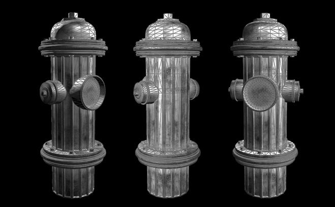
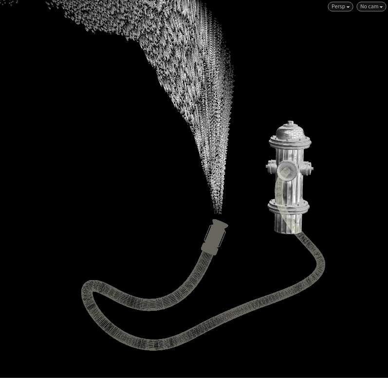
For my geometry, I chose to model a fire hydrant in Houdini and do a wire simulation to get an animating hose.
To get the nozzle of the hose oriented correctly, I created a custom orientation and copied the nozzle so it would animate properly with the wire.
There was one more step because the hose end of the nozzle and the hose didn’t line up perfectly, I had to project the points at the end of the hose onto the nozzle in the direction of the wire’s tangent vector.
TIP
Change the Collision Handling in the Wire Solver to SDF for better looking collisions.
02 Create Particle Source
I isolated a piece of geometry at the end of the nozzle as my source. Scattered points on that geo and made sure they inherited the primitive normals. Then, I put down a Trail SOP and set it to velocity. This creates a vector attribute representing the velocity of the particles. In a wrangle node, I linearly interpolated between the negated velocity and the primitive normal by a random amount for each point.
The code for this is: v@v = lerp(-v@v,@N,fit(rand(@ptnum * @Frame),0,1,ch(“minVariance”),ch(“maxVariance”)));
This step adds variance to the velocities for the particle simulation.
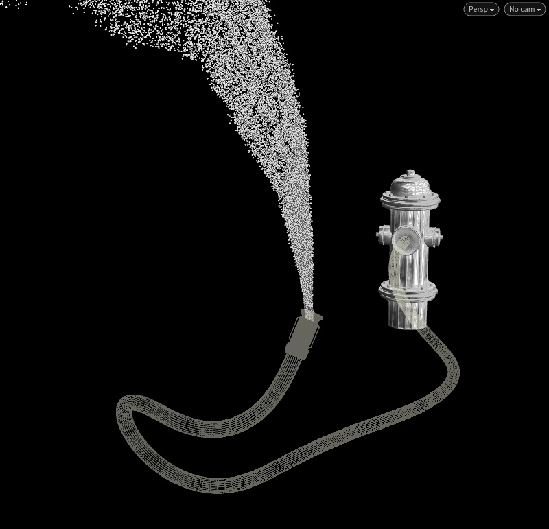
03 Particle Sim
This is where we’ll encounter our first stepping problem that comes about from high speed sources. Put down a popnet and dive in, go to popobject > Birth tab. At the bottom, there are a few menus to choose the interpolation type for the particles. I found that these settings worked for my setup. What this step is doing is interpolating the source between frames, giving us the look we want. I added a few popforce nodes and turned on noise and ramped the amplitude by age to give the particles some more movement; nothing too excessive though.
04 Post Particle Sim Tweaks
One of the more important steps - this is where we’ll shape the particles which will in turn, shape our source volume. Let’s create our first ramp based on age using VEX, in a wrangle we’ll type: @ageRamp = chramp(“ageRamp”,fit(@age,0,ch(“ageMax”),0,1)); and hit the button to the right of the code window to create our parameters. This will give us a ramp as described in this picture, which we can then manipulate by varying the ageMax parameter and the ramp parameter. You can visualize this attribute by adding another line: @Cd = @ageRamp; For clarity, we’ll delete the particles that are older than our max age. We’ll do this by typing in the same wrangle: if(@age > ageMax) { removepoint(0,@ptnum); }
Some particles were going below the ground plane, so I deleted them in a wrangle by writing: if(@P.y < 0) { removepoint(0,@ptnum); } Because I know my ground plane is at origin and aligned to the X and Z axis, this works. If your ground plane was somewhere else and rotated off axis, we would need to know its position, its normal vector and use the dot product to determine which side the particle is situated on the plane.
05 Roll Your Own Motion Blur Ramp
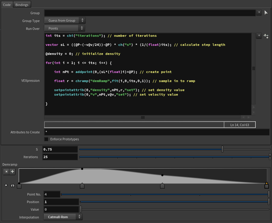
This step may seem a little tricky, but is one that really helps to fill the gaps between the particles between frames. We’ll be explicitly creating motion blur geometry to get the resolution we need for smooth streaks. What is essentially going on in this step, is the creation of particles between where the point was at the last frame and where it is now. We’ll add a ramp to vary a parameter along these streaks. If you copy this code into a wrangle and hit the add parameter button to the right of the code box, you will get immediate results after setting the parameters.
Here’s the code:
int its = chi(“iterations”);
Vector sL = ((@P-(-v@v/24))-@P) * ch(“s”) * (1/(float)its);
@density = 0;
for(int i = 1; i <= its; i++) {
int nPt = addpoint(0,(sL*(floati)+@P);
float r = chramp(“denRamp”,fit(i,0,its,0,1));
setpointattrib(0,”density”,nPt,r,”set”);
setpointattrib(0,”v”,nPt,v@v,”set”);
}
06 Create a Source Volume
Now that we have particles with a density attribute, going from particles to a volume is relatively straight forward, thanks to the fluid source node. Put down the node and go to Container Settings and set the initialize drop down to Source Fuel. Then, in the Scalar Volumes tab, make sure Method is set to Stamp Points. For the most part, this should do, if your volume is still very sparse you can go to the Stamp Points tab and adjust the Sample Distance; be careful not to go very high as it is computationally expensive.
07 Source Advection
To get some extra wispy details in the source volume, I used a volume VOP to advect the fuel and temperature. This is a very deconstructed version of Houdini’s built-in cloud tools. This is essentially the same as adding noise to geometry in an attribute VOP. I like this method more than the built-in noise tools in the fluid source node, as this is an additive process.
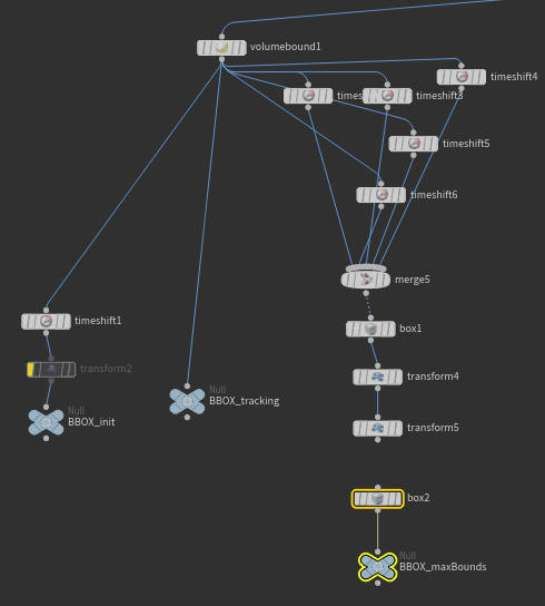
08 Bounding Boxes
Setting up bounding boxes for a pyro simulation is very important to ensure the simulation resizes properly and doesn’t exceed limits. This simulation prep optimizes your scene for simulating efficiently, so that you’re not spending time calculating areas that don’t need to be calculated. The first bbox (bounding box) we set up will be the initial bbox. There’s a node called volume bounds that creates a box that represents the bbox of your source volume. Now that we have our bbox, we’re going to to use a time shift node to shift the source volume to the initial frame. My first frame was frame 6; it’s not always the first frame that you want to use. Then we’ll set up our tracking object bbox - this bbox tells the simulation to always sim at least these voxels. Last and most important is our max bounding box. To set up this bounding box, I like to get an idea of the space the source occupies over time so I do a few time shifts of the volume bounds - one every 50 frames or so - worked well for this. Now that I had a good reference for where my source will be over time, I created a box and placed it based off of the reference, scaling it up some more, so the pyro has room to move about and do its thing.
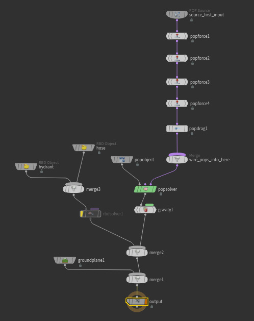
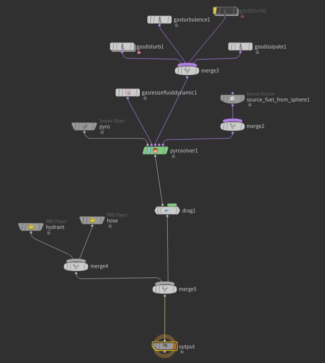
09 Pyro Sim
Houdini’s built-in shelf tool is really nice for setting up the skeleton of our pyro DOP network. I’ll start a new file as to avoid any funny business, put down a sphere and click on the flames button in the shelf tool. Go into the DOP network and copy and paste the pyro object, pyro solver and source volume into the working file. In the pyro object, change parameters so that they look at the initial bounding box. Put down a gas resize node, add the tracking object and the max bounds. Go to the volume source and change it to the source volume. This setup should be enough to hit play and see the pyro simulate for the first time. Next is shaping the look and combustion of the pyro.
Shaping the Look
The pyro node has everything built in to get a nice result, but you can always push things further with micro solvers, which is something I’d highly recommend. Doing so lets you have multiple levels of turbulence, dissipation, etc. I’ll usually always vary the strength of these nodes with fields like temperature and velocity to get variance in the simulation.
Just about every pyro simulation is different, so my best advice is to experiment with each on and off, at high and low values to see how it affects the simulation and create a look with an appropriate mix of these shaping nodes as well as the combustion parameters.
Start Low Res
Make sure to start at low resolutions to get you into the ballpark, then bump up the resolution as you continue to hone in on the look. Continue to repeat this process until you get to your final look.
Depending on how fast your source is moving you may not run into this problem, but I was still getting stepping artifacts even with everything I did to avoid them.
Higher FPS
TIP
Keep in mind that the viewport downsamples all volumes to a max resolution of 256x256x256, so if your volume is higher than this, it’s better to look at renders to gauge the look.
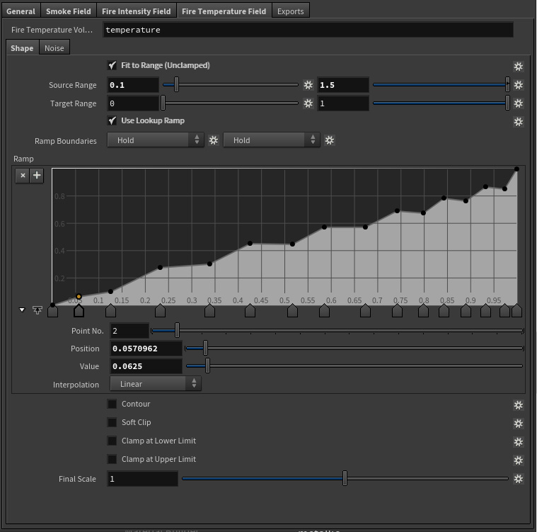
10 Pyro Shading
Houdini’s pyro shader is all you’ll need to make the flames look nice for rendering. The default parameters will give you a good start, but for the most part, you’ll want to make some changes to get the look you’re going for. First use the general tab to get the look started, then go to the smoke, fire intensity and fire temperature field tabs -- I recommend tweaking a lot within these tabs, using ramps to yield non-linear ramps and tweaking the source ranges to get a better look. I find the density of the smoke plays a big role in getting nice contrast in pyro.
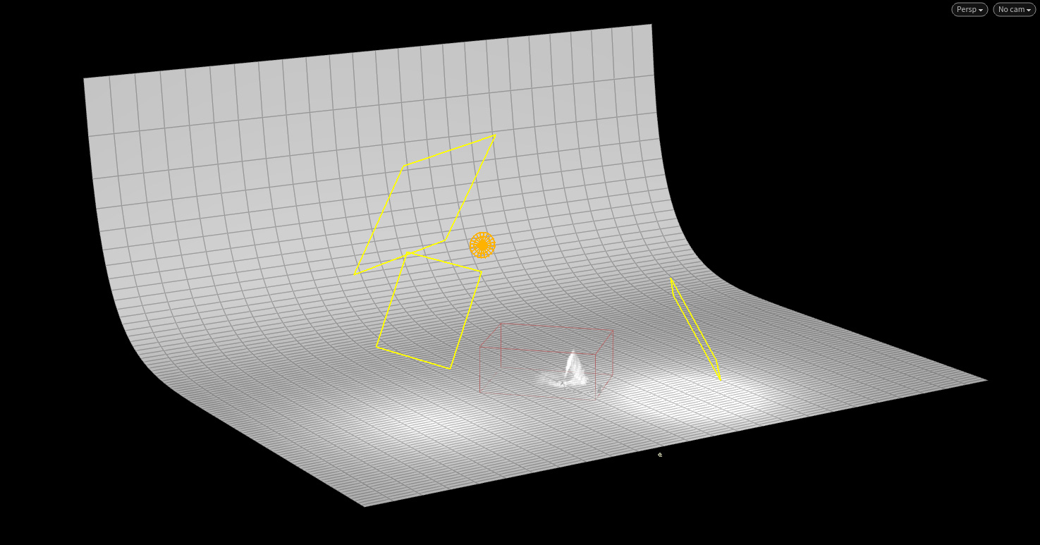
11 Light the Fire
Pyro is self illuminating so the look of the fire is highly dependent on the shading, but lighting is also very important too. You’ll likely notice the effect of lighting on the smoke more than the pyro, though the pyro will be affected as well. I lit this scene with area lights primarily from the side, perpendicular to the camera, I find that side lights add detail to smoke because the self-shadows become more pronounced and expose the finer areas. I also added a rim light and a fill. Then, I created a backdrop and materials for the objects, added an hdri and tuned the lighting to get the look. The fire hydrant’s texture was done by Daniel Siriste.
12 Render Passes
It’s always good practice to render out passes, so that at the compositing step, you can further refine the look. The passes I rendered out for the pyro were the emission pass and the direct lighting passes by light. Then I added all the passes up in comp and further tweaked them with color correction nodes.
13 Compositing
Rarely will you get exactly the look you want in the shader, especially if you’re looking for some secondary effects like glow. I recommend doing some color correction, giving the highlights and shadows some contrast, balance out the hues and saturation to get the look.
Warm Glow
To get a nice glow, I isolated the highlights and blurred them a lot. Then I added this super-blurred out image over the comp at the end and it gave the nice glow. I did it twice at varying levels of blurriness to create a falloff.
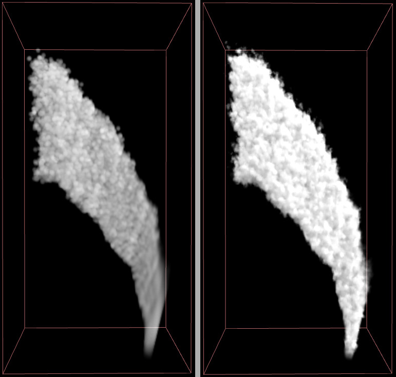
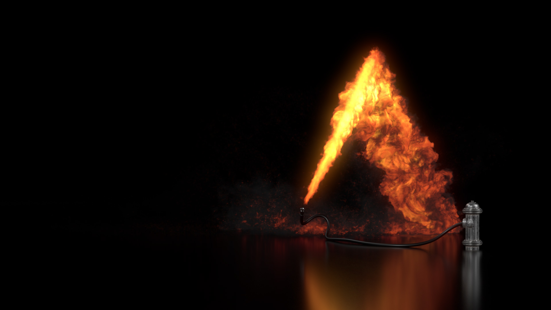
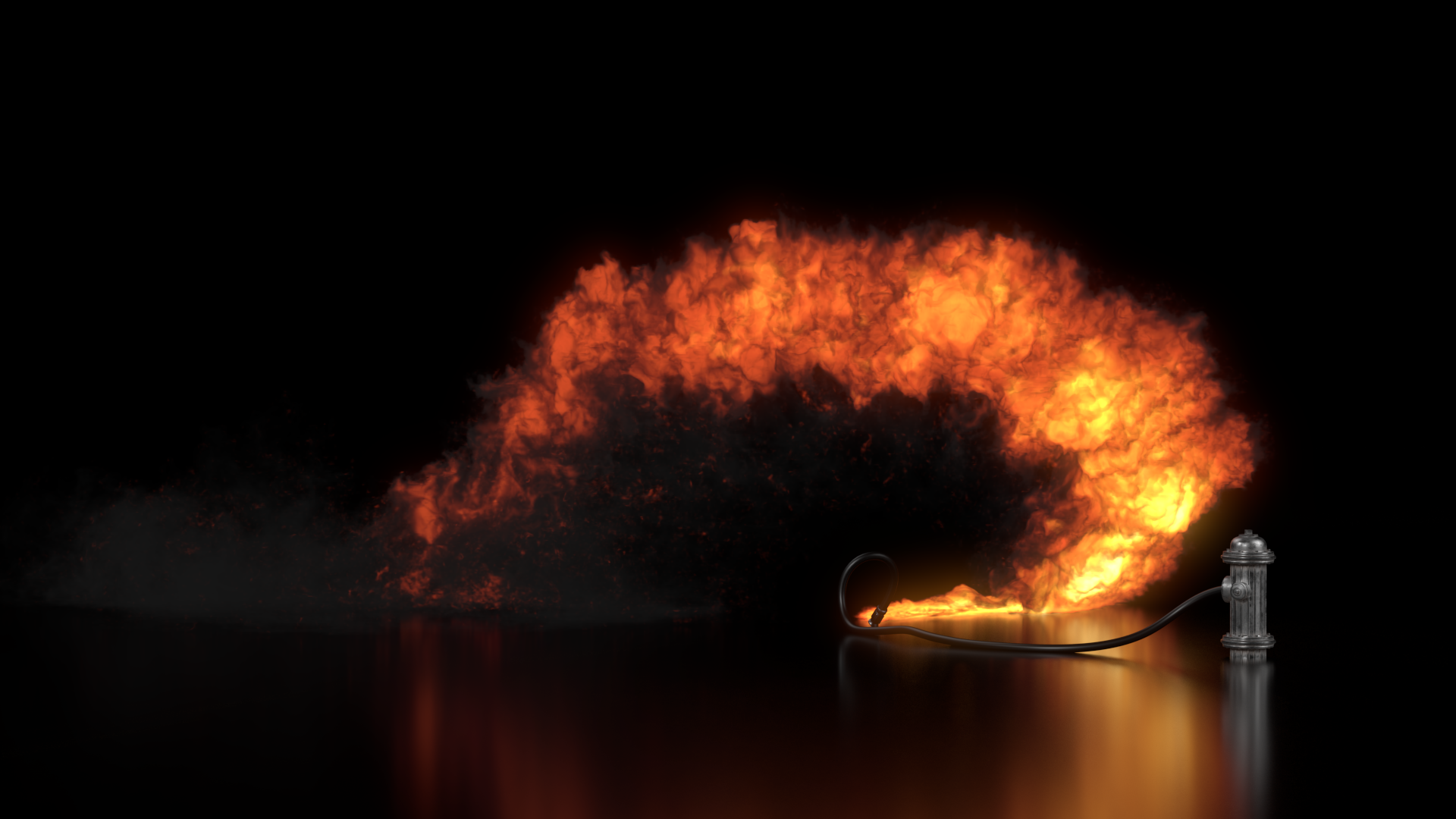
14 GPU OpenCL Pyro vs CPU Pyro
To get a nice understanding of using OpenCL acceleration and what effects it had on the simulation, I did two separate sims with exactly the same settings, shading and post-processing. The look was relatively the same with a few notable differences. What was really noticeable was the difference in time it took to simulate the two versions. The OpenCL simulation took 3 days and is estimated to be 2-3x times faster than the CPU simulation. It was a 720 frame simulation with a max bounds of ~900x600x900 and max size in meters ~9x6x9 taking up ~1.5TB for each simulation. While the look is relatively similar you can observe differences in the images, I prefer the OpenCL version as I find the look to be a bit cleaner, also because it was faster to simulate and took up 20% less space on disk. The GPU I used was the AMD FirePro W9100 (big thanks to AMD for their support in this project!), 32GB of RAM, and an Intel i7-3770 @3.4GHz. Houdini OpenCL pyro does not support multiple gpus. However, the best you can do is point Houdini up and GPU drawing to one GPU and sim and SOP processing and OpenCL calls to a second GPU.
CREATED BY

COMMENTS
craigs 6 years, 7 months ago |
Link to download pyro scene file doesn't seem to be working
AlchemistRS 6 years, 7 months ago |
Thanks,
FYI the download link is doubled just delete the url starting from # back.
trzanko 6 years, 7 months ago |
Fixed! Apologies :D
craigs 6 years, 7 months ago |
fantastic. thanks:)
trzanko 6 years, 7 months ago |
Thanks! Np :D
cpr3danim 6 years, 7 months ago |
Thank You for the breakdown and scene file. Really some very nice work - good comparison of GPU and CPU.
trzanko 6 years, 7 months ago |
Thank you so much! I hope the information is of some use!
annoy4nce 6 years, 6 months ago |
Great work, the comparison and the sim were really good, I'm super envy not being able to set a clean project like you did, thank you very much!!
trzanko 6 years, 6 months ago |
Thank you!
RamaKrishna 6 years, 4 months ago |
How much time it took to sim on cpu?
jorgemartinsegura 6 years ago |
Great work! I have only one question... Why in the wire simulation, in the sop solver only the last point in the wire is were the vel is applied?? thanks
trzanko 6 years ago |
Thanks! It's only applied on the end because the end or the "nozzle" is where most of the thrust force would be coming from
taccuser 4 years, 8 months ago |
Getting lots of "skipping unrecognized parameters" error while loading the project file. Using Houdini 17, please help.
bsilvaLS 4 years, 7 months ago |
Hey! Awesome tutorial, thank you for this!
A couple corrections -- the code *text* in step 05 has a couple syntax errors (the screenshot is correct!). Specifically, "Vector sl = ..." should be "vector sl = ..." and there's a missing ")" on the "int nPt = ..." line.
Also, at least on Windows, when copying the code text from Firefox, it uses different quote characters than the VEX editor, so we had to replace all the quotes to get it to work. Not sure what the solution is for that, but a heads up for others!
thakordipak 3 years, 3 months ago |
awesome tutorial
DJ_Dhrub 2 years, 1 month ago |
Link to the second video please, Seems like that's broken. Can someone please update the link, Or give any alternate link?
Please log in to leave a comment.