| On this page |
The ML Deformer 20.5 content library example was built entirely using the example-based ML nodes released with Houdini 20.5. The scene files and ML cache can be downloaded from the Content Library.
This setup applies ML to animation. It demonstrates how ML can learn from quasistatic simulation to improve over linear blend skinning. This type of simulation is usually more expensive than linear blend skinning. However, providing a sufficiently large data set of simulated examples allows the ML model to train and approximate the simulation results efficiently and accurately. This works even for unseen poses that are not part of the data set.
This application of ML falls into the category of regression; ML is used to approximates a function. In this case, the function maps each given rig pose to a simulated deformation of the skin.
Stages 
The ML Deformer 20.5 setup consists of three main stages:
-
data set generation
-
ML training
-
inference (applying the trained model).
Each of these stages is comprised of smaller steps, which can be found in several different subnetworks. The data set generation stage uses mostly ML nodes whose names start with ML Example. The ML training and inference stages relies mostly on ML nodes whose names start with ML Regression.
Data set generation 
The data set generation stage consists of the following steps:
-
input generation
-
computing targets
-
pre-processing.
Each of these steps are in SOPs but controlled from a TOP network.
Input generation 
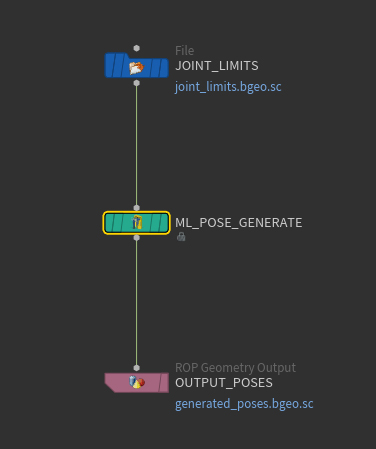
Each input is a random pose. It is assumed that each joint of a pose stores only a rotation (the translation part is not used and assumed to be zero). A collection of input poses is generated using random sampling from ![]() ML Pose Generate. Generating the random angles from the full 360 degree range is an ineffective strategy. Instead, each joint is assigned a random angle chosen from an appropriate range, determined from a set of representative animations. These angle ranges are provided as joint limits on the input of
ML Pose Generate. Generating the random angles from the full 360 degree range is an ineffective strategy. Instead, each joint is assigned a random angle chosen from an appropriate range, determined from a set of representative animations. These angle ranges are provided as joint limits on the input of ![]() ML Pose Generate.
ML Pose Generate.
Computing targets 
For each randomly generated input pose, a corresponding target skin deformation must be generated. This process consists of two separate, smaller steps:
-
perform a quasistatic simulation to obtain a deformed tet cage
-
use the deformed tet cage to deform the skin.
For each given input pose, a deformed tet cage (tetrahedral mesh) is obtained using a quasistatic simulation. This happens in the pose cages subnetwork of the ML Deformer. Before this simulation starts, the tet cage is rotated and translated so it’s globally aligned with the input pose. After that, several simulation time steps are performed during which the aligned rest pose is gradually linearly blended toward the input pose. At each time step, the interpolated pose is used to deform the anatomical bones that act as constraints for the simulation.
For further processing, each input pose is combined with its corresponding deformed tet case (target). A collection of labeled examples is formed using ![]() ML Example, each having the input pose as the input component and the resulting tet cage as the target component. The simulation step is frame-dependent so each labeled example is fetched individually from the TOP level using a
ML Example, each having the input pose as the input component and the resulting tet cage as the target component. The simulation step is frame-dependent so each labeled example is fetched individually from the TOP level using a ![]() ROP Geometry Output (rather than using a SOP-based for loop). From these separate labeled example files, a single file for the collection of all labeled examples is formed using File Merge in combination with another
ROP Geometry Output (rather than using a SOP-based for loop). From these separate labeled example files, a single file for the collection of all labeled examples is formed using File Merge in combination with another ![]() ROP Geometry Output.
ROP Geometry Output.
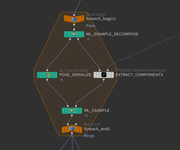
The ML approach learns from the vertices of deformed skins rather than tet cages. This means each deformed tet cage needs to be converted to a deformed skin. The next step transforms the collection of labeled examples to a new collection where each target component is a deformed skin instead of a tet cage. This happens in the pose_skins network of the ML Deformer. A SOP for loop transforms each of the labeled examples from the previous step. Within the For Loop SOP, ![]() ML Example Decompose breaks up each labeled example into its constituent input and target components. The packed primitive representing the input component is kept as is without copying its embedded geometry. The tet cage target deforms the skin which results in a new type of target called deformed skin. The existing input and the new target type are then bundled again using
ML Example Decompose breaks up each labeled example into its constituent input and target components. The packed primitive representing the input component is kept as is without copying its embedded geometry. The tet cage target deforms the skin which results in a new type of target called deformed skin. The existing input and the new target type are then bundled again using ![]() ML Example.
ML Example.
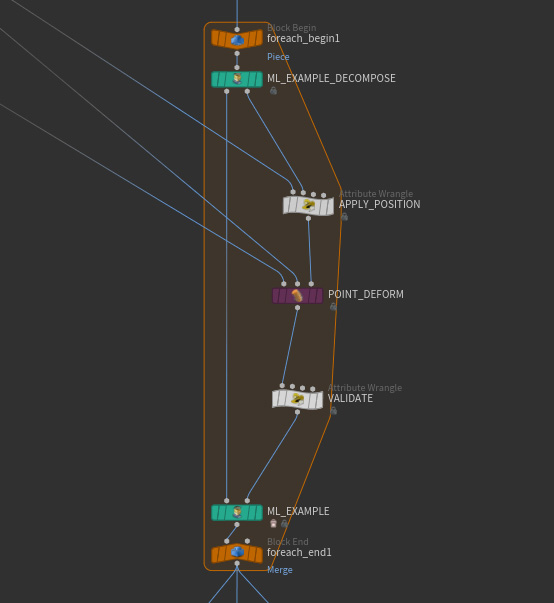
Besides transforming the labeled examples, this step also discards outliers using the validation mechanism provided by the example-based ML nodes. A validation step is performed each time the skin is deformed. If the skin contains NANs (bad numbers), then the skin is marked invalid using a detail attribute recognized by the ![]() ML Example. This results in an empty output and discards the example. Each input and each corresponding target are always bundled together in a single labeled example. This means no indexing problems result from this validation step.
ML Example. This results in an empty output and discards the example. Each input and each corresponding target are always bundled together in a single labeled example. This means no indexing problems result from this validation step.
Pre-processing 
Before the start of pre-processing, each labeled example has a pose as its input component and a deformed skin as its target component. If a deformed skin has 50,000 points, then you would need 150,000 floating-point numbers to store the full skin deformation. Training a neural network that has an output layer of 150,000 units can be quite expensive. Such a model may be costly to inference as well. To fix this, the pre-processing steps aim to reduce the size of the the targets used for training.
The preprocessing stage consists of two smaller steps:
-
computing skin displacements relative to the rest position
-
approximating these skin displacements using principal component analysis (PCA).
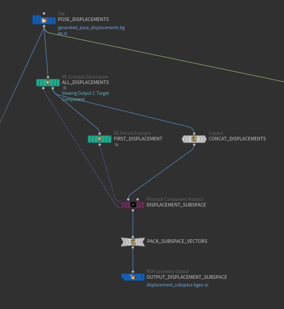
The first pre-processing step is similar to the conversion of a deformed tet cage to a deformed skin in the previous stage. It applies a transformation to the target while leaving the input unchanged. The first pre-processing step converts each deformed skin to a displacement that is relative to the LBS-animated (linear blend skinning) skin in rest space. This happens in the sub-network pose_displacements. For each combination of a pose and a deformed skin from the previous stage, the pose comuputes the difference between the deformed skin and a skin deformed using LBS. This results in a skin displacement relative to the deformed skin. The inverse of LBS is applied to each displacement vector, resulting in a skin displacement relative to the rest skin. This new representation of the skin deformation as a displacement relative to the rest position has the advantage of being independent of the global position and orientation of the input pose.

The second pre-processing step uses a principal component analysis to approximate the rest displacements using a much smaller representation. This happens in the data_set network. From all the skin displacements in the collection of labeled examples, a new and much smaller set of skin displacements is formed using ![]() Principal Component Analysis. In Analyze mode, each original skin displacement can be accurately approximated using a linear combination of the new ones. ML Deformer 20.5 uses only 128 of these coefficients, which allows you to have a neural network with only 128 outputs instead of the original 150,000. This number 128 can be changed.
Principal Component Analysis. In Analyze mode, each original skin displacement can be accurately approximated using a linear combination of the new ones. ML Deformer 20.5 uses only 128 of these coefficients, which allows you to have a neural network with only 128 outputs instead of the original 150,000. This number 128 can be changed.
The final data set for training is assembled using another For Loop SOP, where an incoming labeled example has a pose as its input component and a skin displacement as its target component. Each pose is converted into a point float attribute using ![]() ML Pose Serialize. Each skin deformation is converted into its 128 PCA components using
ML Pose Serialize. Each skin deformation is converted into its 128 PCA components using ![]() Principal Component Analysis, in Project mode. The resulting examples are written out as a data set for regression training using
Principal Component Analysis, in Project mode. The resulting examples are written out as a data set for regression training using ![]() ML Example Output.
ML Example Output.
Training 
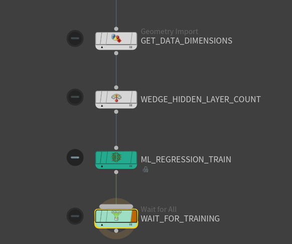
The TOP network COOK_RECIPE creates the entire data set and performs the training. This network ensures all the steps outlined above, plus the training stage, are executed in the right order.
The data set for regression training is read at the TOP level by the training node ![]() ML Regression Train. The TOP setup performs multiple training sessions, each with different hyperparameter settings. There is only one specific hyperparameter you train here: the number of hidden layers of the neural network. Each invocation of ML Regression Train writes out its result to a separate model file.
ML Regression Train. The TOP setup performs multiple training sessions, each with different hyperparameter settings. There is only one specific hyperparameter you train here: the number of hidden layers of the neural network. Each invocation of ML Regression Train writes out its result to a separate model file.
Inference 
The inference stage is the stage where the trained neural network can be used to predict skin deformations for unseen poses. The ML Deformer H20.5 content library example performs inference in two distinct places:
-
an analysis network that allows the performance of the model to be evaluated.
-
an APEX setup that allows the trained model to be tried on various user-controlled poses
The analysis network can decide which trained model performs the best. The separate posing scene file with APEX nodes illustrates how a trained model can be incorporated into an animation workflow.
Analysis Network 
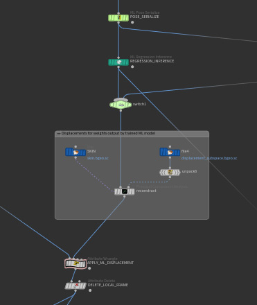
The network analyze_trained_model uses ML Regression Inference. ML Regression Inference may refer to any of the models generated by ![]() ML Regression Train.
ML Regression Train.
ML Regression Inference applies the trained model to inputs. These inputs can be seen inputs which were included as input components of the data set. They can also be unseen inputs that are not part of any example of the data set. ML Regression Inference takes its inputs and computes its outputs in the same format included as inputs and targets in the data set. This means if you want to apply ML Regression Inference to an input pose, ![]() ML Pose Serialize must be applied to that input pose first. The output of ML Regression Inference consists of PCA components. These PCA components are converted back to a skin deformation using the inverse of the steps that are applied to each skin deformation in the pre-processing stages:
ML Pose Serialize must be applied to that input pose first. The output of ML Regression Inference consists of PCA components. These PCA components are converted back to a skin deformation using the inverse of the steps that are applied to each skin deformation in the pre-processing stages:
-
compute a skin displacement from the PCA components
-
apply the skin displacement to the deformed skin.
The analysis subnetwork also allows the results of both linear blend skinning and the machine learning model to be compared to the ground truth. This allows you to see how accurate the model is on trained poses. It also allows you to see how accurate the model is on poses outside the training data set using ground truths generated separately for those unseen poses.
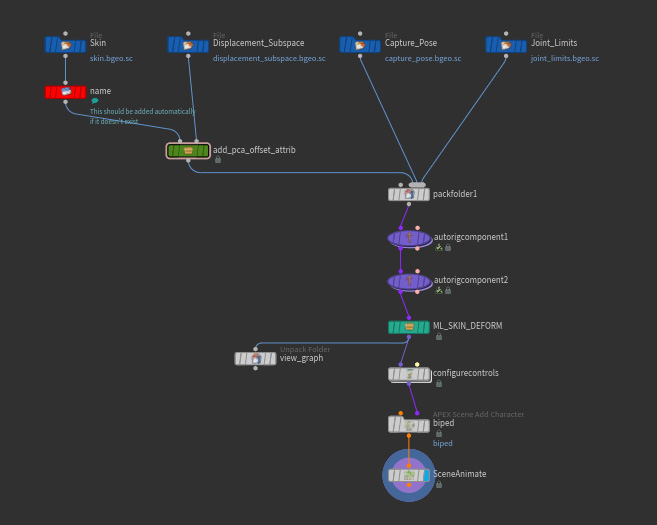
APEX Setup 
There is a separate scene file pose_using_ml.hip that allows you to pose a trained model. It uses two assets that help automate the translation from the PCA components generated by the ML model to deformed skins. You can manually modify the input pose and see what the skin deformation predicted by a trained ML model looks like.