ML GROOM DEFORMER

Introduction

This is a tutorial on how to use the example-based machine learning (ML) nodes that were released with Houdini 20.5 to build a groom deformer. This scene demonstrates how a variety of ML setups can now be built entirely from within Houdini just by putting down ML nodes and setting parameters, without the need to write custom training scripts. The tutorial is an addition to the corresponding project files released in the content library. You can download them here!

The system is based on the ML Deformer H20.5 and  extends the functionality to work with grooms. 

This is one of the projects I presented at the Houdini HIVE Horizon event hosted by SideFX in Toronto. You can watch the full presentation here:

PCA Shenanigans and How to ML | Jakob Ringler | Houdini Horizon

This text tutorial dives into more specific setup details.

General Idea

In essence, the goal is to predict how fur deforms on a character or creature using a machine learning model, instead of relying on expensive simulations and procedural setups.

The Problem

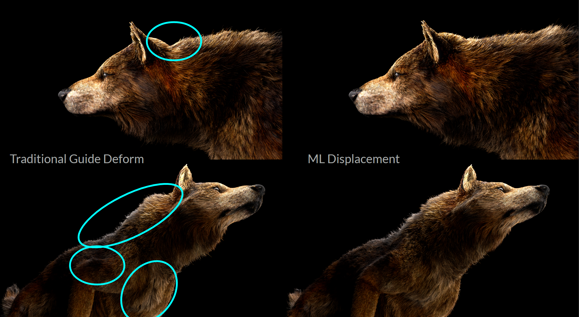
There are a few common issues when deforming hair naively or linearly. Particularly around the joint areas, there are numerous intersection problems, where hair above the joint pierces through the fur layer below (see the second position below). Ideally, we want to see a nice layering of guides and better volume preservation. Achieving this can be computationally expensive and often requires a simulation along with one or more post-processing steps to get right.

Left to right: Rig - Default Guide Deform - Ideal Deformation (Quasi-Static Simulation) - Rest Guides - Displacement in Rest Space

The Solution

Our goal is to predict the deformation that needs to be applied to the guides based on the rig position using an ML model. The model learns to map from the rotation data of each rig joint to the approximated displacement of the guides for each pose. 

To do this, we need a substantial number of examples for the model to learn from. The general pipeline looks something like this:

Data Generation

To generate all the training data, we need 2 things to start out with:

Joint Limits

This could be a fixed degree value on each joint (e.g., 30) or, preferably, if we have a few motion clips for the rig, we can procedurally configure the joint limits based on the range of motion present in our clips. To do this, use the configure joint limits SOP.

Pose Randomization

In Houdini 20.5, a new node was introduced to streamline this process. The ml pose generate SOP takes existing joint limits and generates random poses in a Gaussian distribution. This means there will be more normal poses than extreme ones, which is desirable for training a model that performs well in common positions.

The output is a bunch of posed packed rigs stacked on top of each other.

Simulation Loop

In this stage, we run over each of our generated poses using TOPs and generate/simulate a good guide deformation result accordingly. 

This step could be almost anything. There is just a few limitations:

The result has to be deterministic / procedural / quasi-static!

That means we can't have any inertia (think jiggle, overshoot, simulation goodness) and we should always get the same result when we rerun the same inputs. Additionally, the relationship between inputs and outputs should be smooth; similar inputs should yield closely related results. So, we should avoid any methods that might lead to wildly different outcomes for nearly identical inputs.

In this case, we are using a combination of a quasi-static tet simulation and a de-intersection pass, in which the guides are advected through a velocity field built from the hair and skin.

Create Pose Blend Animation

Quasi-Static Tet Simulation (Vellum)

De-Intersection through Velocity Advection 

Ground Truth Examples

Calculate Rest Displacement

We need to then move each of these poses back into rest space using the default guide deform SOP. In rest space, we compute the difference of each point on the  deformed guides to the rest guides using the shapediff SOP. This gives us a clean point cloud, we will store together with the rig position as one training example.

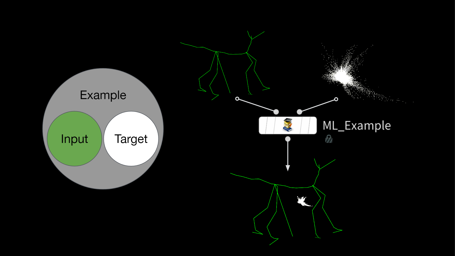
Storing the Examples

Once all of the poses are simulated and the displacement is generated, we can start assembling what is called an ML Example in Houdini. Usually this is called a data sample. It consists of an input and a target and is one of the many examples we show the network during training to make it (hopefully) learn the task at hand.

PCA Subspace Compression and Serialization

After generating all of our pose displacements, we bring in those points and merge them all together and calculate our PCA subspace.

Creating the Subspace

We let PCA do the math magic and compress our 4000 examples down to fewer components. In this case we can think of it as inventing new, but fewer blendshapes of the original displacements that (if combined correctly) can reconstruct all of our inputs accurately. 

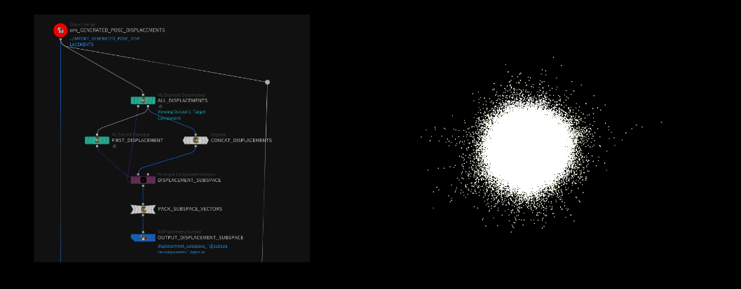
This PCA-generated point cloud is all of the new components (invented blend shapes) stacked on top of each other. They aren't separated in any way in Houdini (not packed, no ids or anything). We determine which points belong to each component by understanding the size of the sample. For example, if our dataset contains 100,000 points, we can identify the components by examining the list of points. The first component consists of points from 0 to 99,999 (ptnum 100k-1), while the second component includes points from 100,000 to 199,999 (ptnum 200k-1), and so forth.

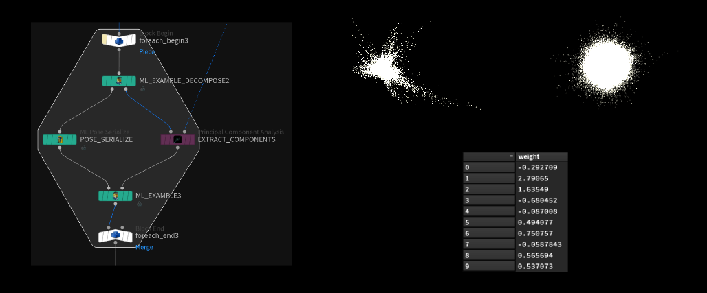
Calculating the Weights per Example

The reconstruction will never be 100%, but we can reach 95%+ levels while using only a few hundred components.

Why Do All This?

Instead of having to learn 100.000 point positions (300k float values), we only need the model to predict the weights needed for reconstruction (64, 128, 512, 1024 floats or whatever we choose). The size of our network stays small and training and inference is much faster that way. 

Performance would also suffer immensely, trying to map a few joint rotation values to a giant list of point position values.

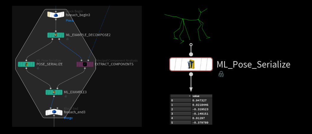
Serialization

On the other side of that for loop, we serialize the joint transforms using the new ml pose serialize SOP. All this node does is take the 3x3 matrices stored on each joint and map the values to a -1 to 1 range and store each float of that matrix on a single point in series. We end up with a long list of float values which represent our joint rotation data. This is necessary because neural networks don't like matrices as a single input. It's easier to only work with single float values. The mapping to the -1 to 1 range makes sure it plays nicely with activation functions inside the network.

Data Set Export

After postprocessing all the examples, we can write out the full data set to disk. The ml example output SOP stores all the samples together in a single data_set.raw file, which will be read by the training process later on.

Training

The training is completely done inside of TOPs. There isn't too much to it after having done all that preparation work, which does the heavy lifting and is the process that takes the most amount of time (to setup and to run all the simulations as well).

ML Regression Train

The core of the whole system is the ml regression train TOP, which is a wrapper around PyTorch under the hood. We can set all the common training parameters on there and it comes with some nice quality of life features, such as splitting our dataset automatically in training and validation data based on a ratio we can specify. 

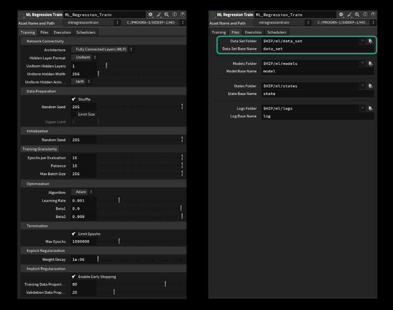
We can also control all the parameters of the network (called hyperparameters). The most important ones are:

Wedging

Having all those parameters available on the node in TOPs opens the door to do some wedging! This is common practice and is usually called hyperparameter tuning. We could run multiple experiments to find the right combination of parameters that give us the best performing model. The parameters I mentioned above are a good place to start wedging. For the groom deformation example here, I only wedged the amount of layers and the size of each layer.

Inference

Or doing everything in reverse..

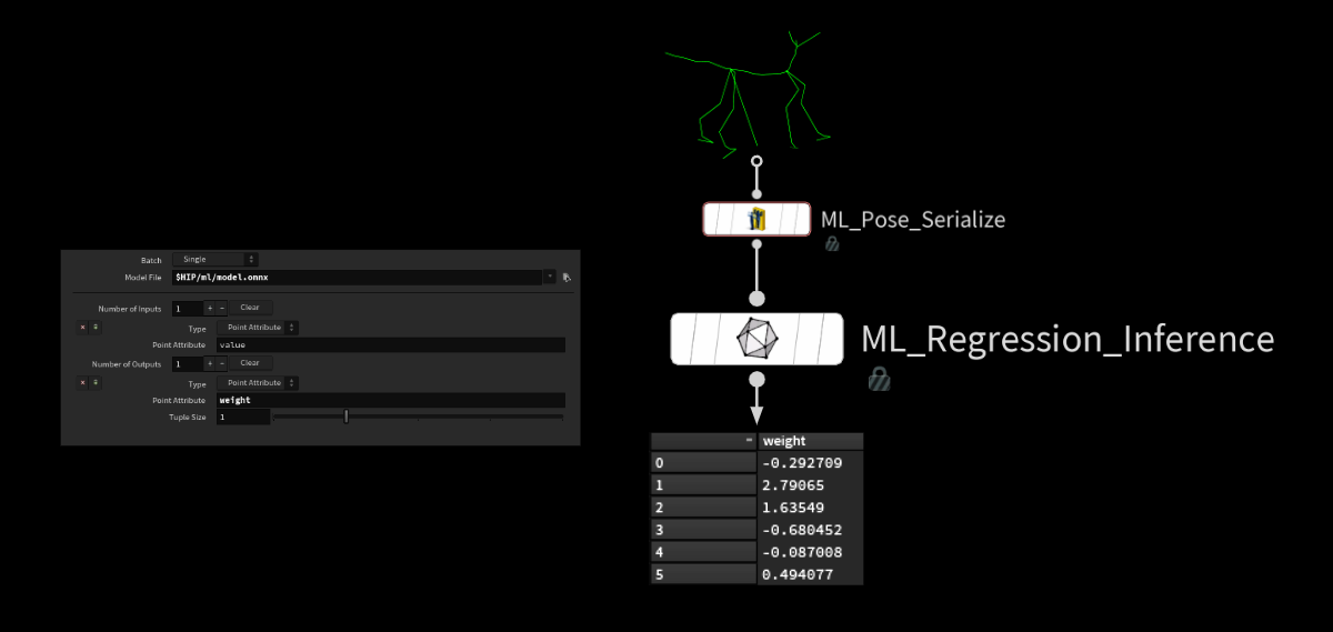
The model then spits out a list of weights, which we can use to reconstruct our displacement based on the subspace components we saved earlier.

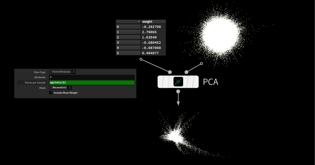
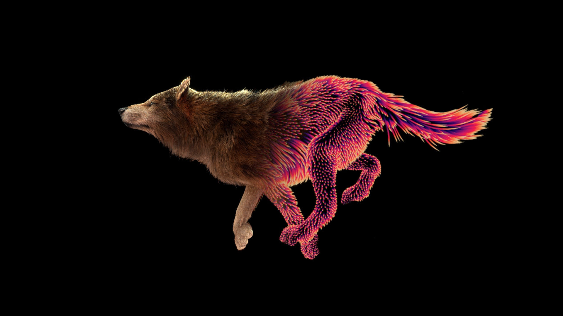
Feed those two into a PCA node and let it do it's thing. This gives us the displacement we need to deform the guides. The rest should be pretty straight forward. Apply the predicted displacement to our guides by adding each vector to the corresponding point on the curves.

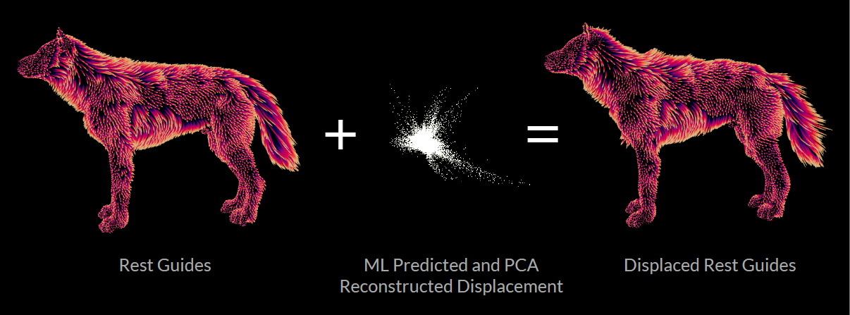
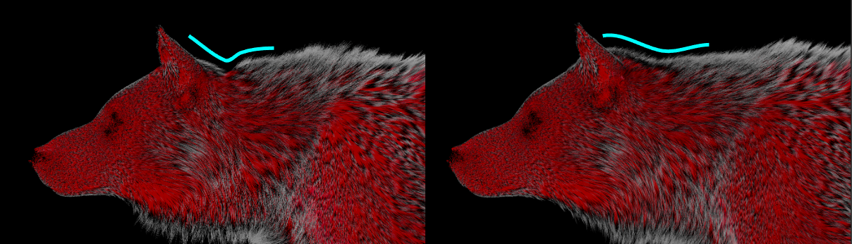
That gives us a jagged looking ruffled up wolf. But if we deform it into the correct position the displacement is based on we get a smooth looking result.

Here's a frame by frame preview where I blend back and forth between the original linear guide deform and the ml prediction.

 We can also measure and visualize the error of our prediction. The number is the Root Mean Squared Error (RMSE) of all the point differences. The color visualizes the local error compared to the ground truth on the right.

Results

Here's a few more screenshots and renders of how this could affect a full groom:

Credits

Thanks to the amazing team at SideFX for all the help with this project!