はじめに
このチュートリアルでは、Houdini 20.5 と同時にリリースされた、サンプルベースの機械学習 (ML) ノードを使って、自分の描いたドローイングを Houdini に理解させる方法を解説していきます。シーンを見れば、ML ノードを配置してパラメータを設定するだけで、訓練用のカスタムスクリプトを書かずとも、Houdini 内で様々な ML セットアップを構築できるのがわかるでしょう。このチュートリアルは、Content Library 内でリリースされたプロジェクトファイルの補足として作成されたものです。このページからもファイルをダウンロードできます。
このプロジェクトは、トロントで行われた SideFX 主催の Houdini HIVE Horizon イベントの際に筆者が発表したプロジェクトの1つです。講演の全容はこちらでご覧になれます。
PCA Shenanigans and How to ML | Jakob Ringler | Houdini Horizon
以下のテキストで、より具体的なセットアップの詳細を解説しています。

概要
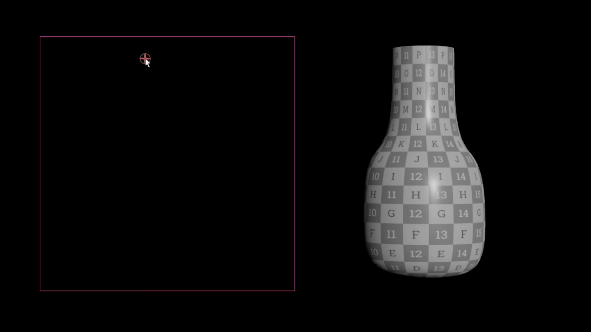
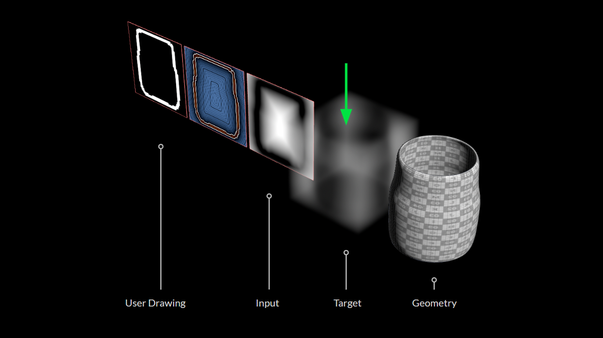
大きな目標は、キャンバス式のドローイング UI を使ってジオメトリ生成をコントロールすることです。ここで主な問題になるのは、適切なトポロジはおろか、メッシュを予測させるだけでも極めて困難であることです。ニューラルネットワークは、グリッド状データのトポロジを入出力として取ることを好みます。
配列や画像、ボクセルボリュームの形を使うとうまくいきます。そのいずれかを使い、大きさが固定されていると、訓練時の入出力として比較的使いやすいでしょう。この時 Houdini のプロシージャルなワークフローが力を発揮します。望ましいオブジェクトを作るための HDA やその他のタイプのジェネレータのセットアップを作成すれば良いからです。ジェネレータを駆動するパラメータに、シルエット状のドローイングをマッピングすることを ML モデルに学ばせることで、適切なオブジェクトをプロシージャルに生成していきます。
グリッド状の浮動小数点値による画像 --> 配列状の浮動小数点値
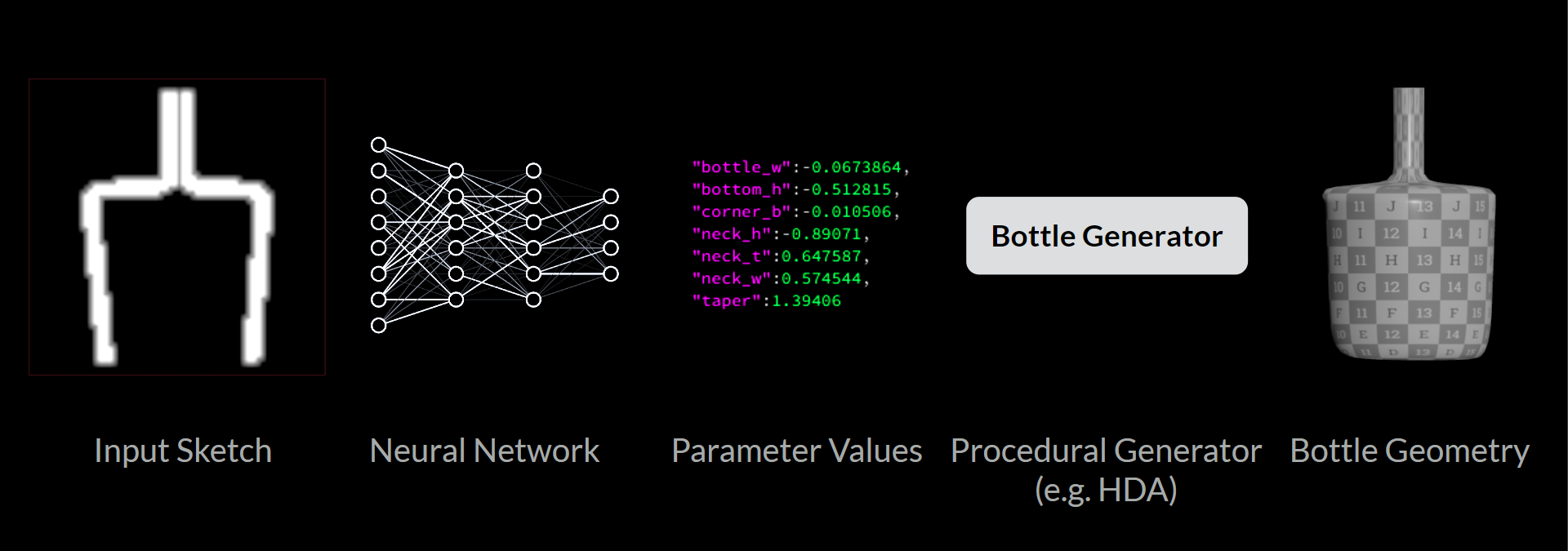
これにより、ジオメトリの予測に伴うあらゆるリスクや面倒を回避します。このアーキテクチャには、後述するような様々な長所や欠点がありますが、大部分は、モデルに何が出力できるかという制約が明確である、キャンバスの解像度が小さくても過度な制約を受けないなど、どちらかと言えば利点に類するものです。
- 何が入力されても、常に合理性のある結果を返す
- ジェネレータを使うと、必ずしも入力ドローイングに描かれていないディテールまで作ることができる
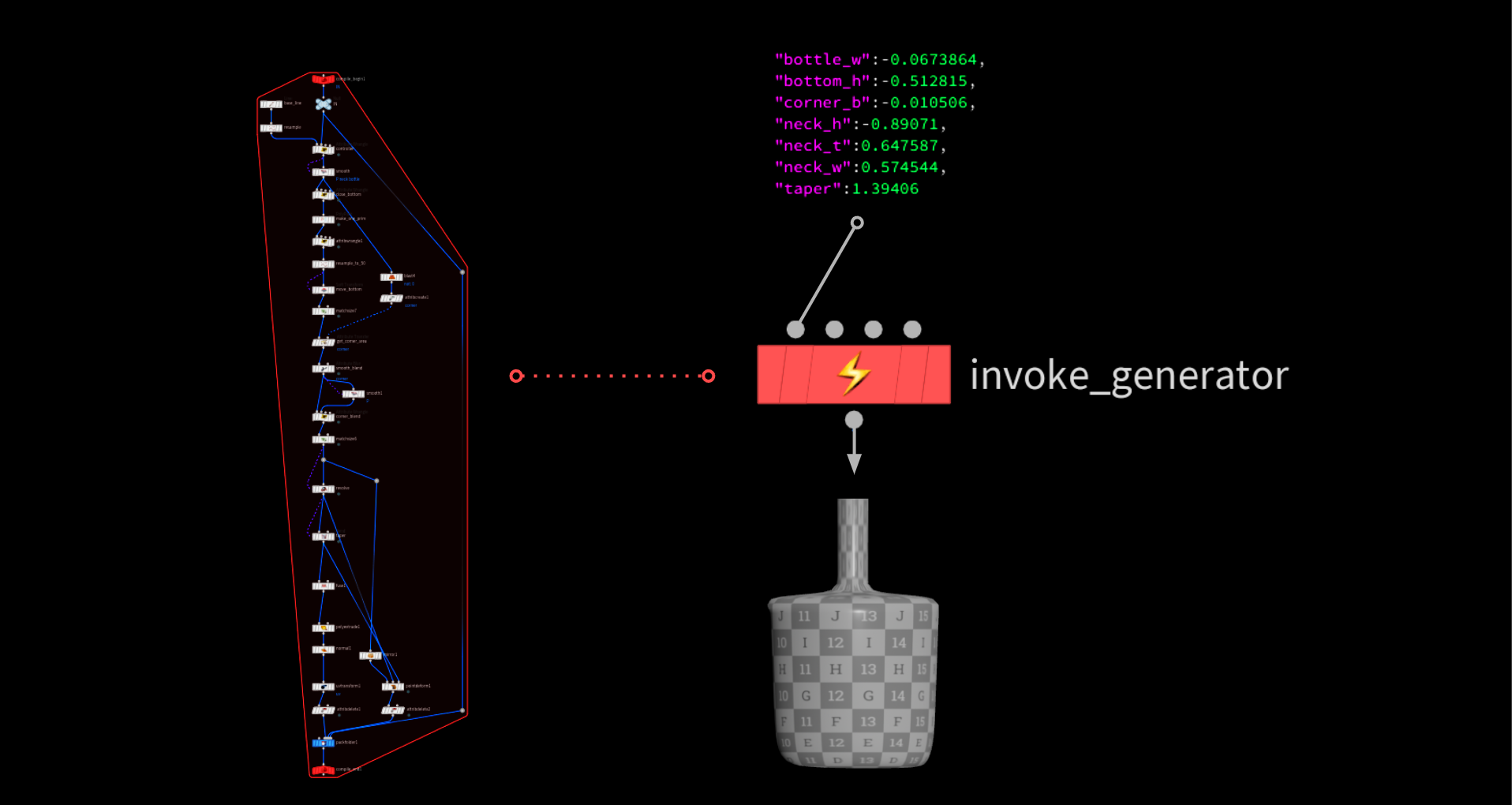
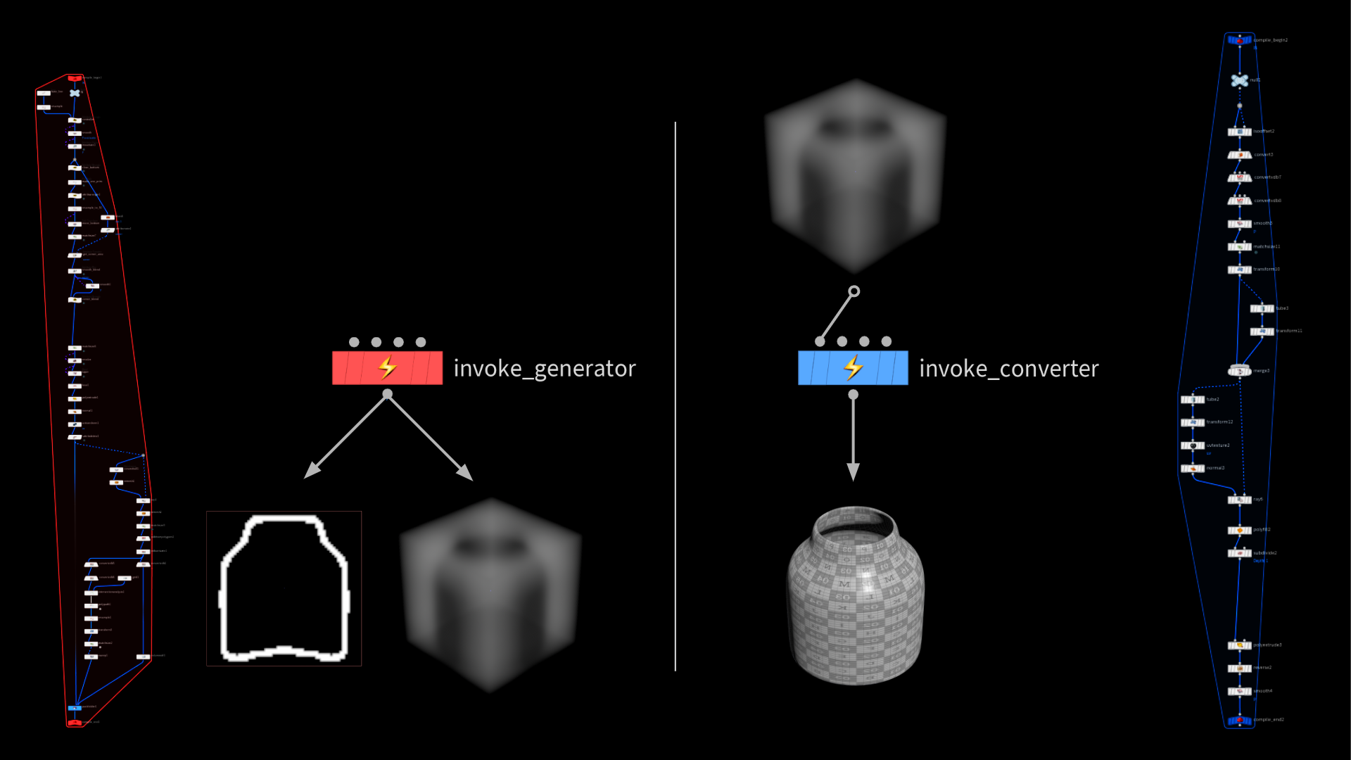
ジェネレータ
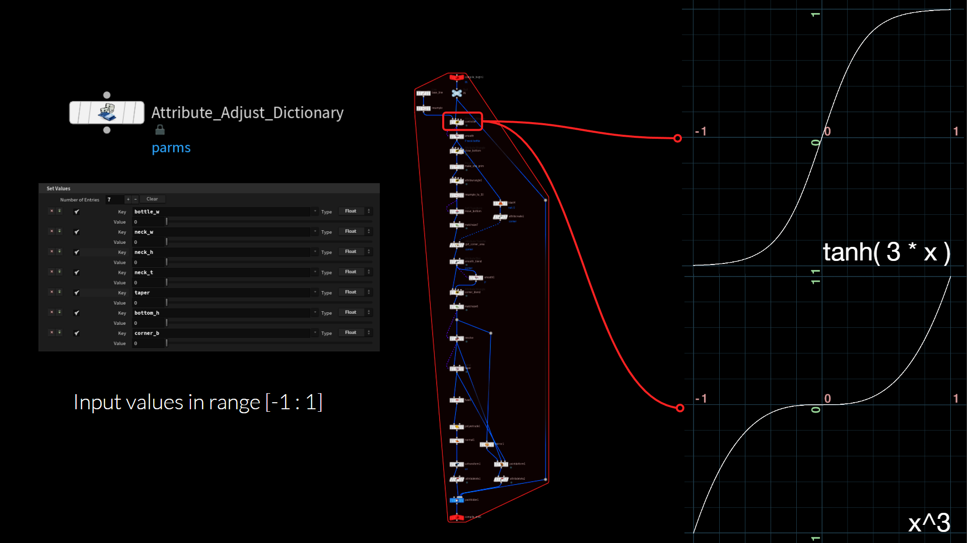
ここでは、利便性と流用性を考慮し、コンパイルしたブロックを使用します。これにより、複数の場所でセットアップを実行できると同時に、ブロック内機能のライブ編集も可能になります。これには通常、HDA を使用できます。
パラメータは、Dictionary アトリビュートに格納してコントロールします。この辞書をブロック内に読み込み、しかるべきノードに値を振り分けます。
訓練を簡素化するため、パラメータの値があまり広範に散らないようにします。全ての値の入力を、-1 から 1 の中に収めます。これは、良い基準値になるだけでなく、ネットワーク内で使用される tanh() のアクティベーション関数とも合います。
後ほどジェネレータをランダム化する際に乱数値の分布を制御できるよう、パラメータの入力値は、シグモイド関数および三次関数によってリマップされます。三次関数は、ゼロ付近により多くの値を集中させるのに対し、シグモイド関数は -1 から 1 の上限と下限の方に、より多くの値を押しやります。
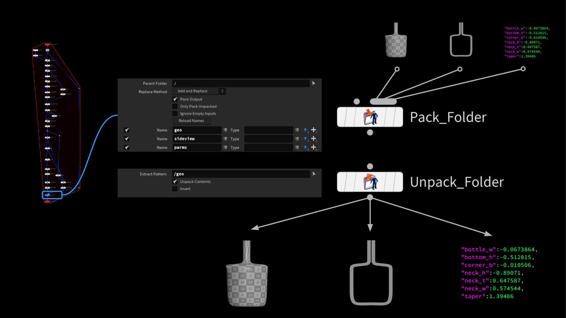
もうひとつ、あまり評価されていないものの楽しい機能として、APEX / キャラクタワークフローの一環として導入された Pack Folder と Unpack Folder があります。異なるジオメトリのストリームをひとつに格納したり、フォルダ名を元に後から再分割する際、大いに重宝します。たいへん便利で、主に、ジオメトリ上に即席の辞書構造を作成することを可能にします。
データ生成
ML グルームデフォーマのデモでは、TOPs でデータを自動生成しましたが、今回は簡単な For Each Loop で全てを実行しています。各サンプルを1秒以下で生成できるうえ、 全ての Houdini セッションを TOPs で立ち上げると作業が滞るため、この方が合理的です。必要なサンプルの生成時間と量によっては、両方の手法を同時に用いるのが良いかもしれません。
単一ワークアイテム内に大量のサンプルを生成し、同時に複数のインスタンスを実行します。
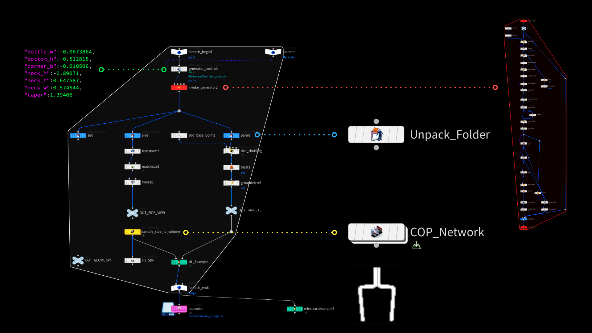
ジェネレータは単なるコンパイルしたブロックであるため、入力辞書のランダム化が必要です。この際、ごく簡単な detail 関数を使って、現在のイテレーションを元に各値をランダム化します。同じ値が重複しないよう、各パラメータには異なるオフセット/シード値を設定するようにしてください。
次に、Invoke Compiled Block SOPでジェネレータを実行し、統合したジオメトリを吐き出させます。これには、先述の Unpack Folder SOP を使うとアクセスできます。後は、データを若干整理し、画像プレーン上のアウトラインをラスタライズした後、機械学習サンプルとしてパラメータ値のリストと一緒に格納するだけです。
その工程を繰り返して 10,000 個のサンプルを生成し、ディスク上に格納します。
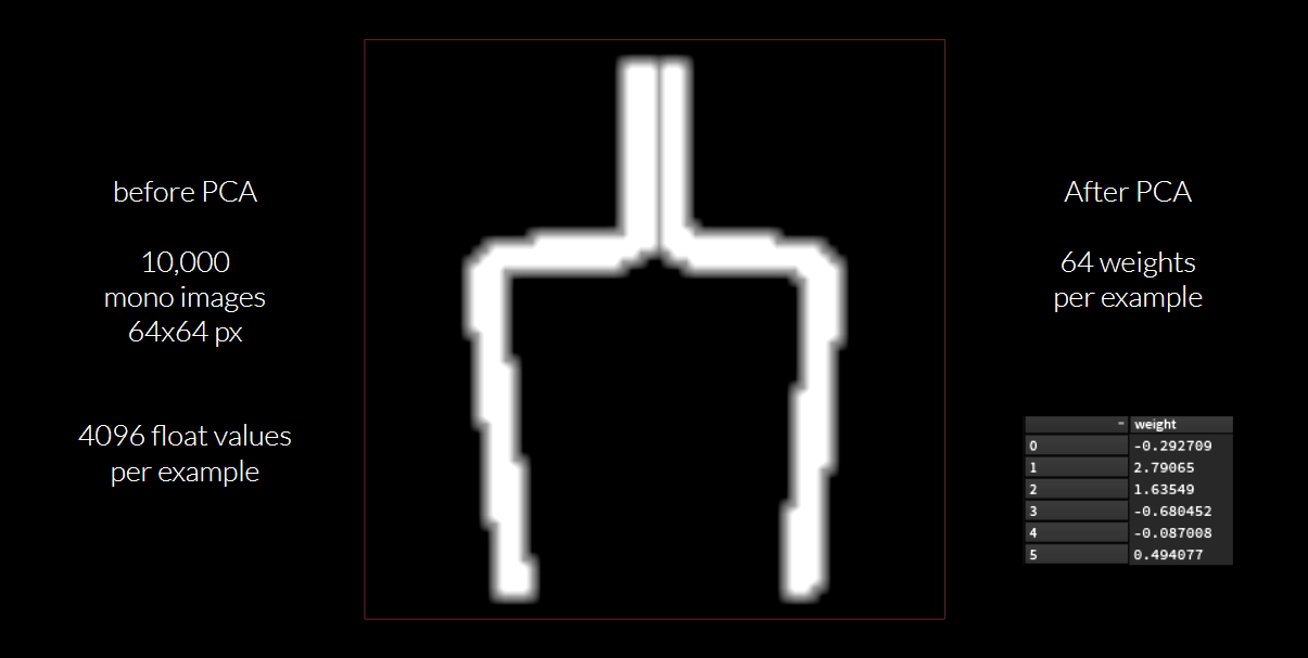
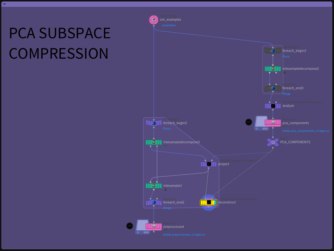
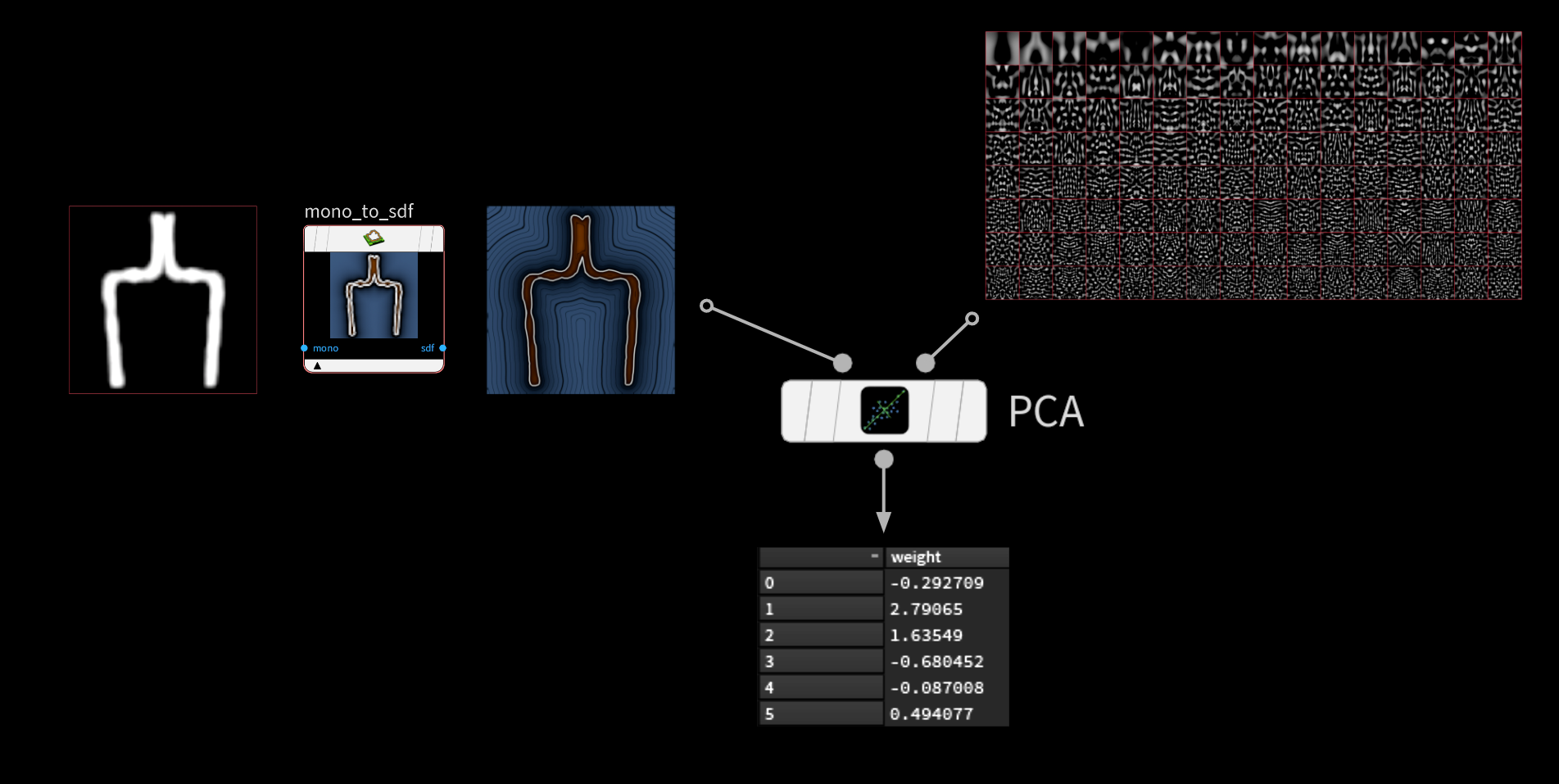
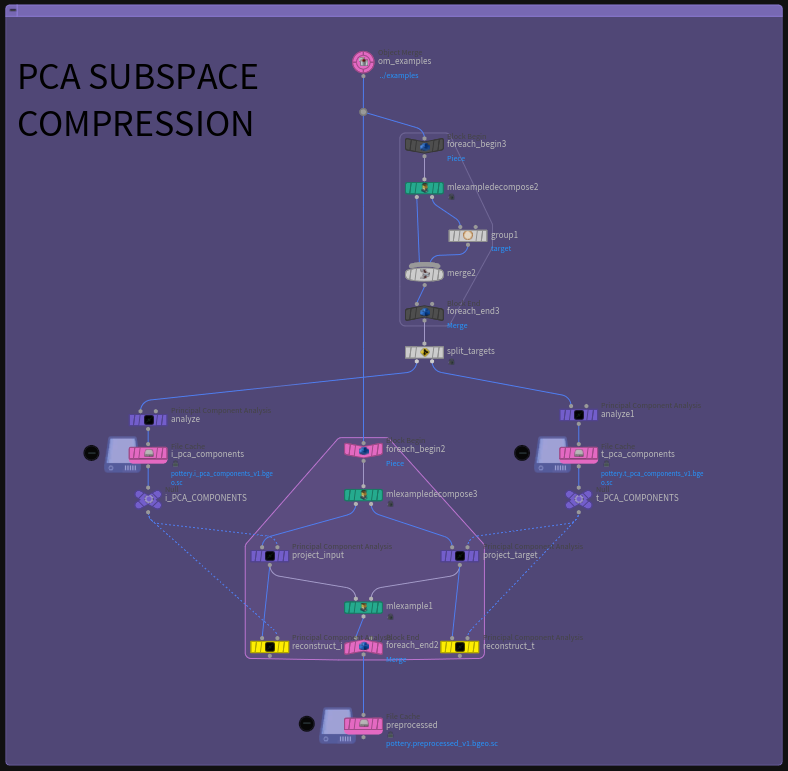
PCA サブ空間の圧縮
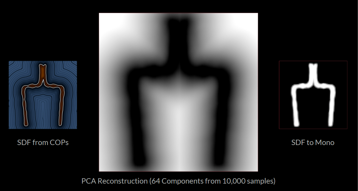
ML グルームデフォーマのプロジェクトでは、PCA を使って全ての変位サンプルをより小さいサブ空間に圧縮することで、ジオメトリ全体ではなく各サンプルのウェイトのみを格納しましたが、今回も入力画像に対して同じ手法を使います。64 x 64 ピクセルの画像を格納するということは、4096 の浮動小数点値の配列をひとつ、ニューラルネットワークに流し込むことになります。ここでは 10,000個のサンプルの画像空間を圧縮し、はるかに少ない数のコンポーネントにします。
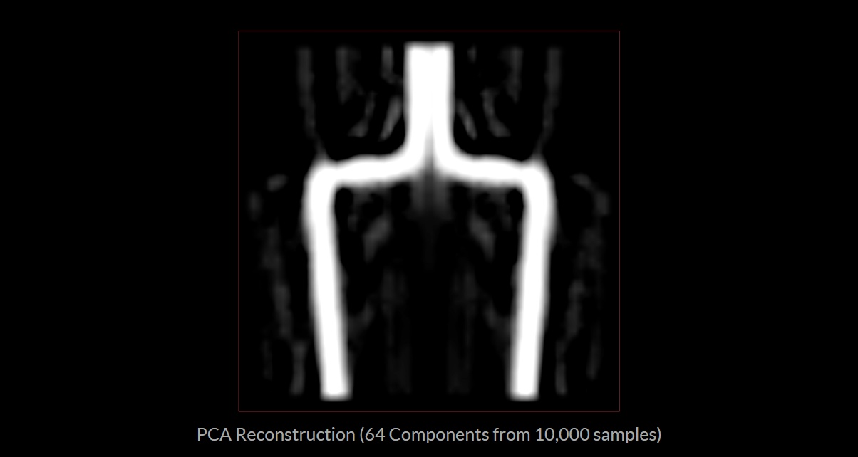
これは理想的な結果ではありません。ボトルの形は判別できますが、周囲に波打ったノイズ的なゴーストが発生しています。コンポーネント数を大幅に増やすのは、有効な改善方法ではありません。
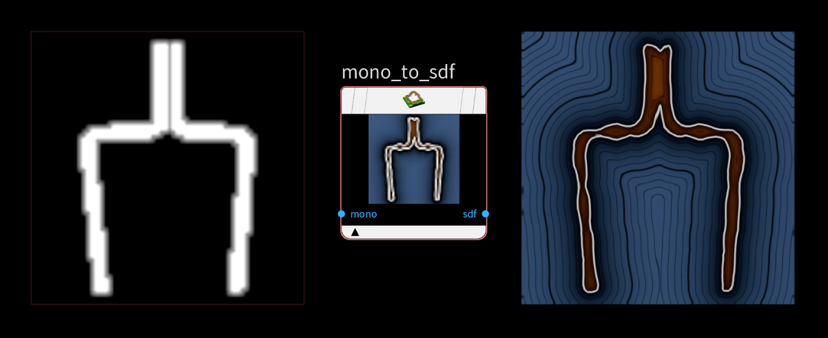
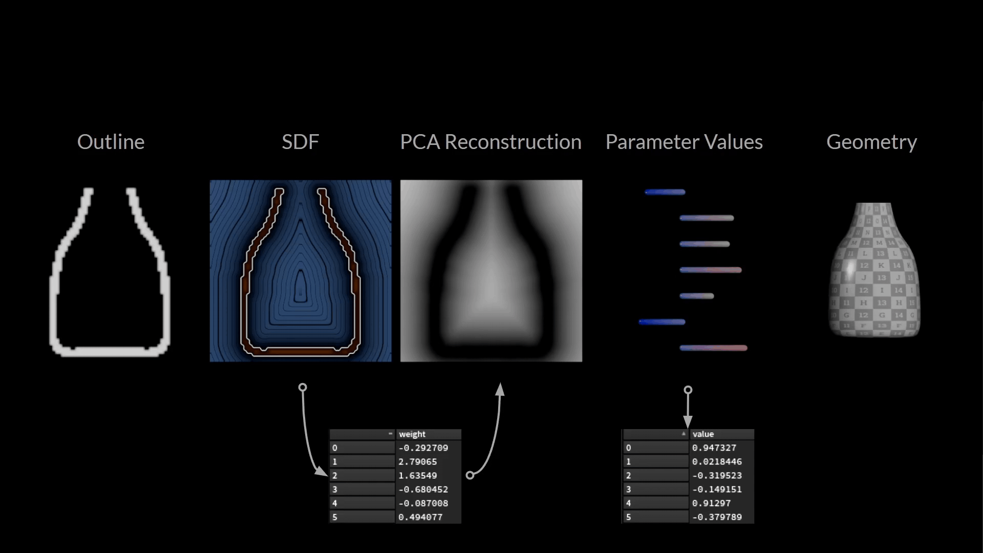
そこで大いに力を発揮するのが、COPs SDF ツールで白黒マスクを SDF に変換するという方法です。この方法を使うと、0 か 1 以外の値も扱えるようになり、ボトルのアウトライン周辺にスムーズで段階的な減衰を適用することができます。
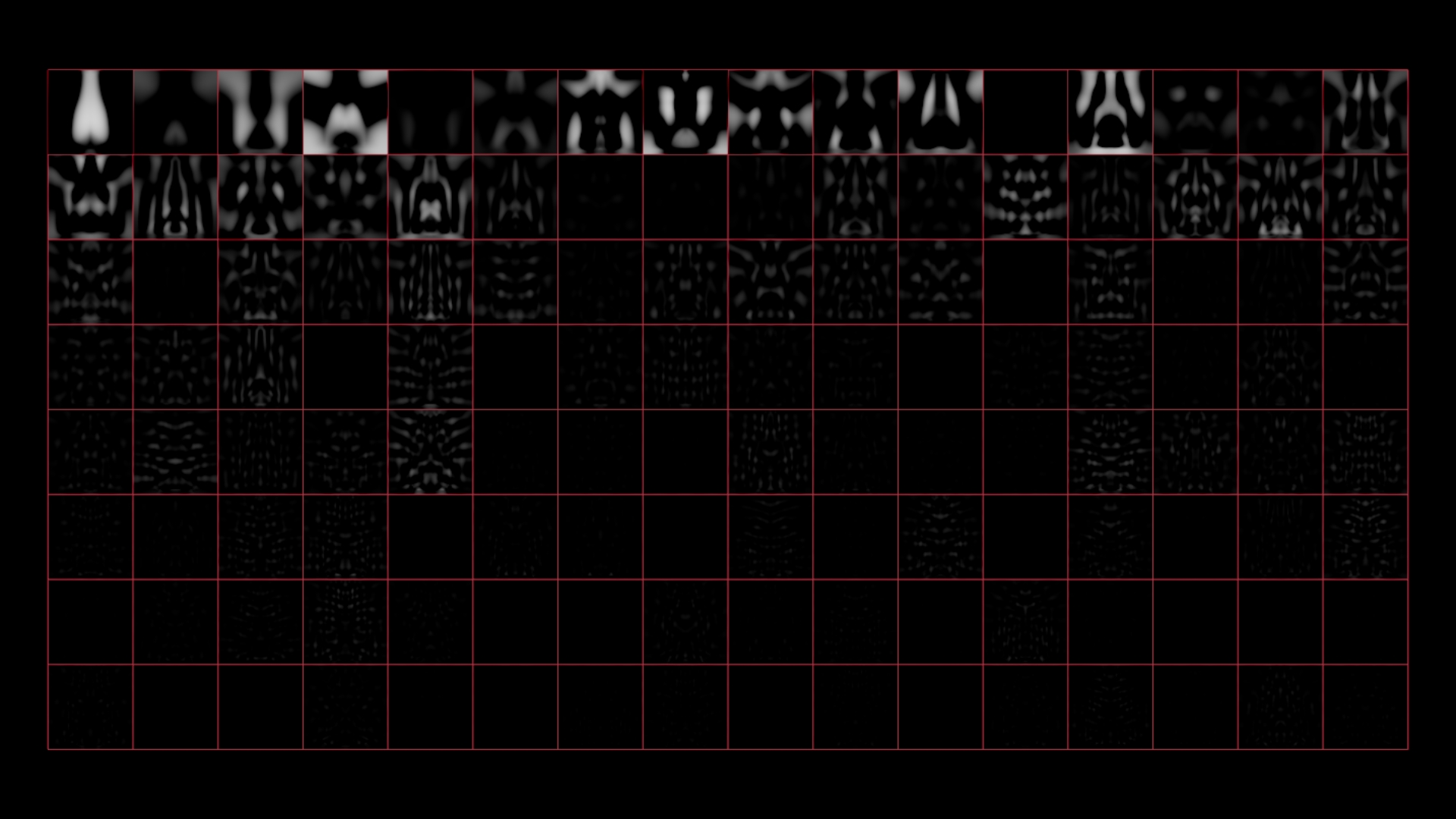
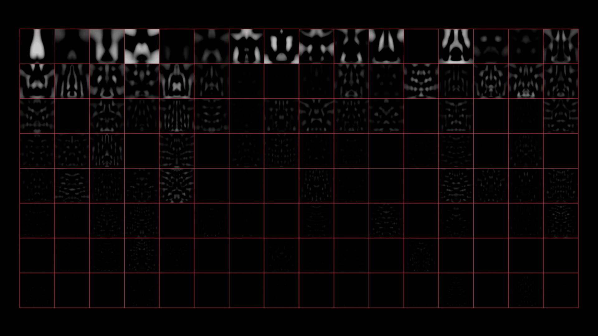
PCA による画像圧縮には、各コンポーネントを視覚化できるという優れた副次効果もあります。
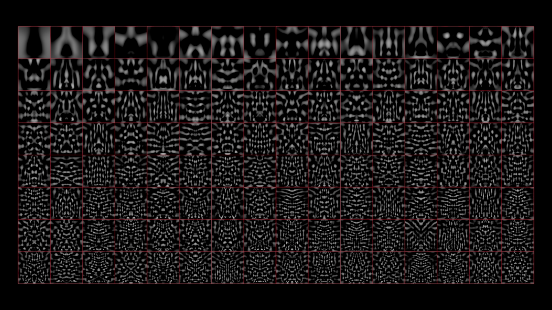
コンポーネントの配列は重要度を元に決まります。そのため、再構築時の影響力が薄れる前の段階では、各コンポーネントに格納されている実際の情報量を確認することができます。左上ではまだボトルの形を認識できますが、右下ではほぼノイズです。
「ほぼ」です。
出典 (画像): List of Physical Visualizations; Dragicevic, Pierre and Jansen, Yvonne; 2012; https://dataphys.org/list/chladni-plates/
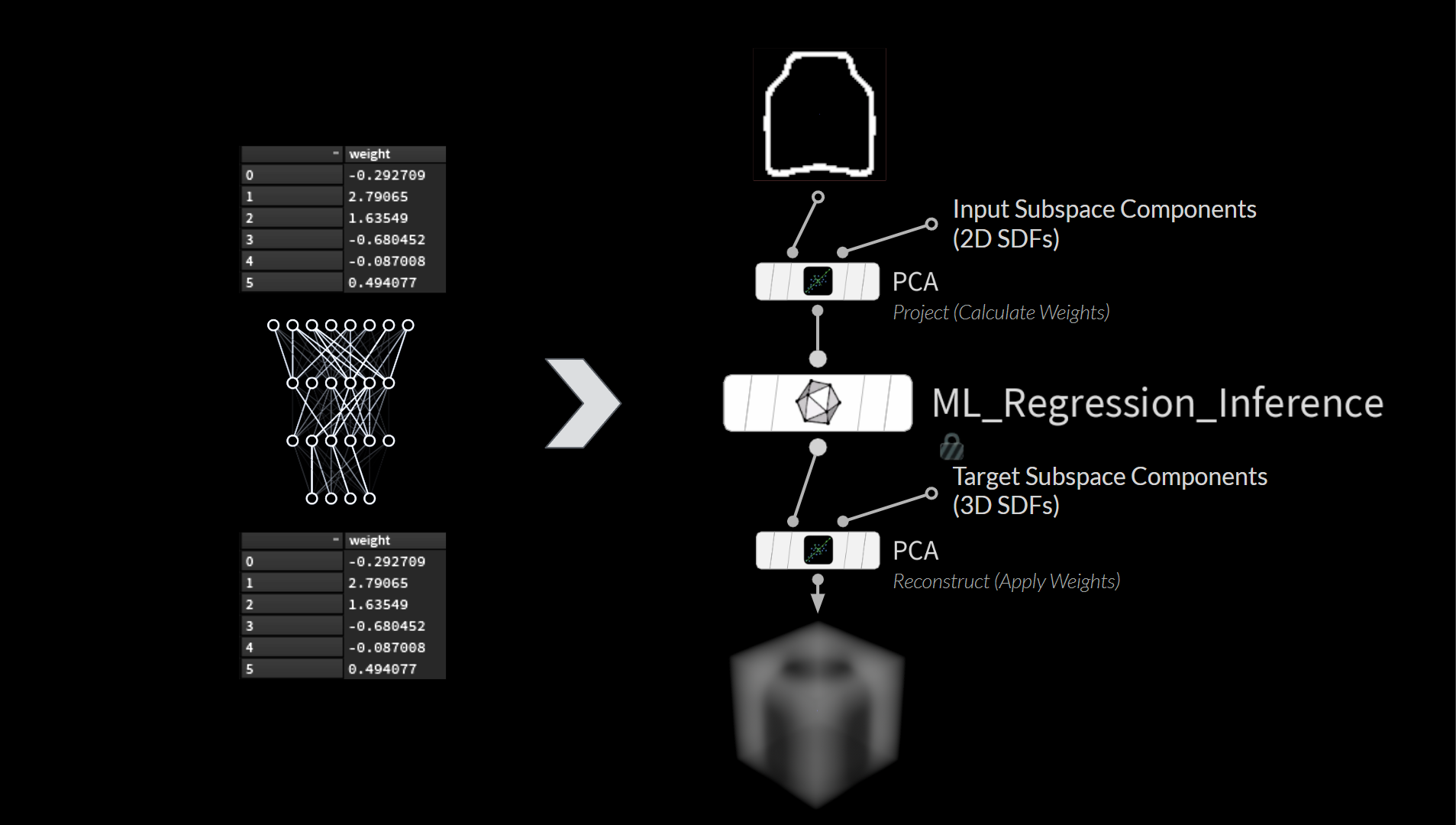
見た目の整った合理性的なコンポーネントがあると、与えられた入力を再構築する際のウェイトの状態も視覚化することができます。
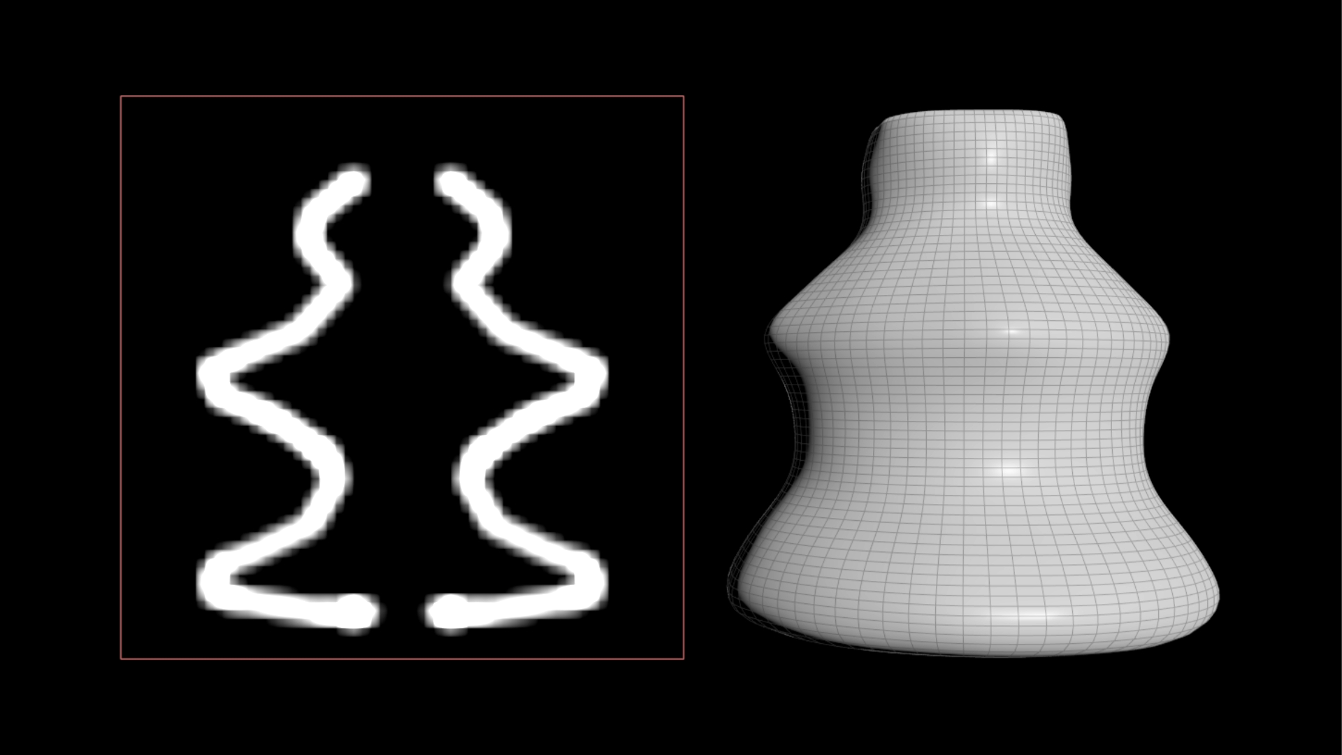
例えば、ユーザが以下のような形を描いたとします (これは見えないところで SDF に変換されます)。
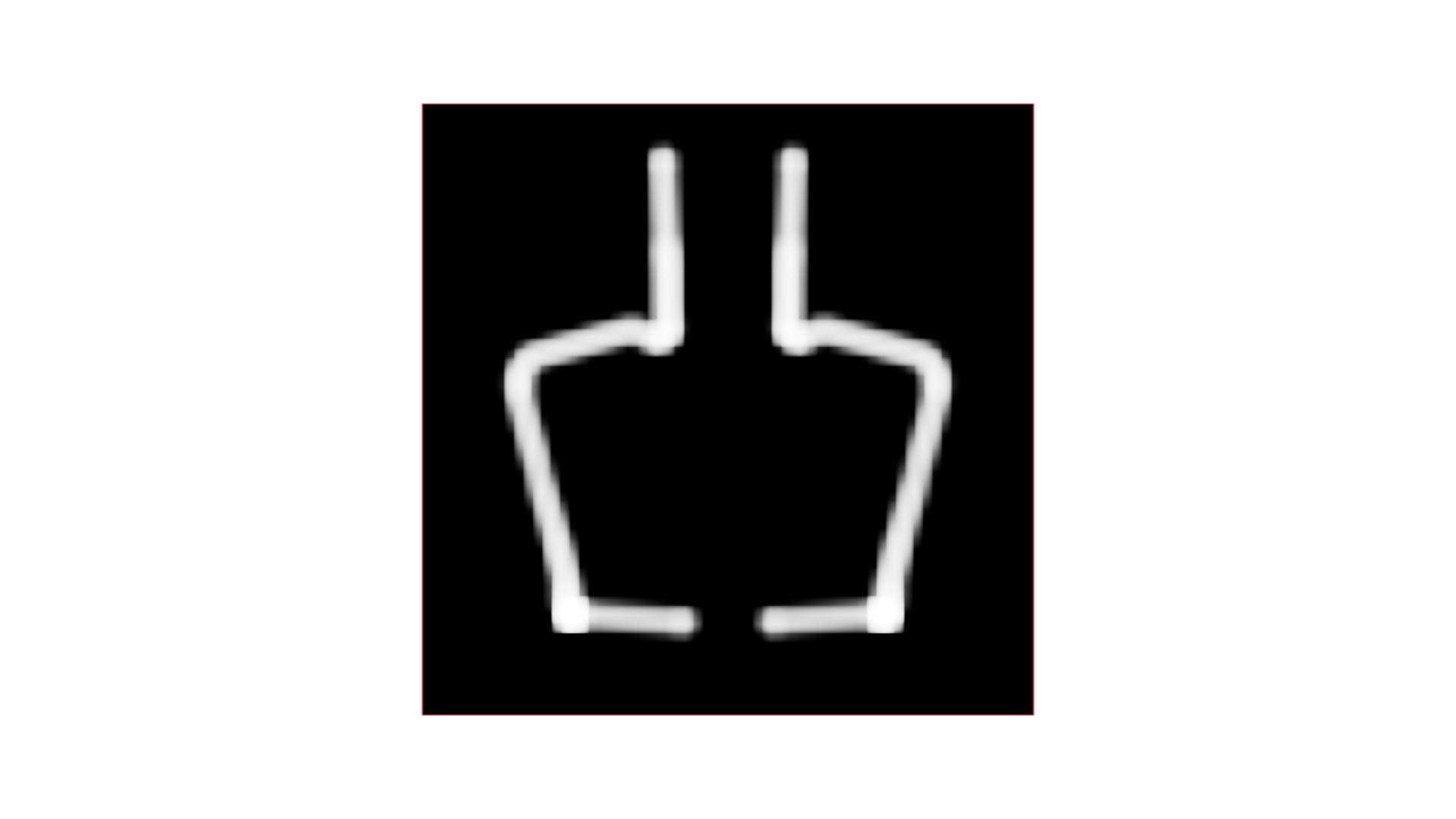
この絵を、事前に計算したサブ空間のコンポーネントと一緒に PCA SOP にフィードすると、それぞれに見合ったウェイトを得られます。このウェイトを、それに対応するコンポーネントに適用すると、最終的な再構築が、どのコンポーネントによって構成されているのかを詳しく見ることができます。
それらを全て足すと SDF の再構築の完了です。幸い、何の問題もないようです。
まとめ:このようにごく少ないウェイトで作業できることで、4096 の浮動小数点値を使わずとも、64 の入力値 (PCA のウェイト) によって、8個のジェネレータパラメータへのマッピングが可能になります。
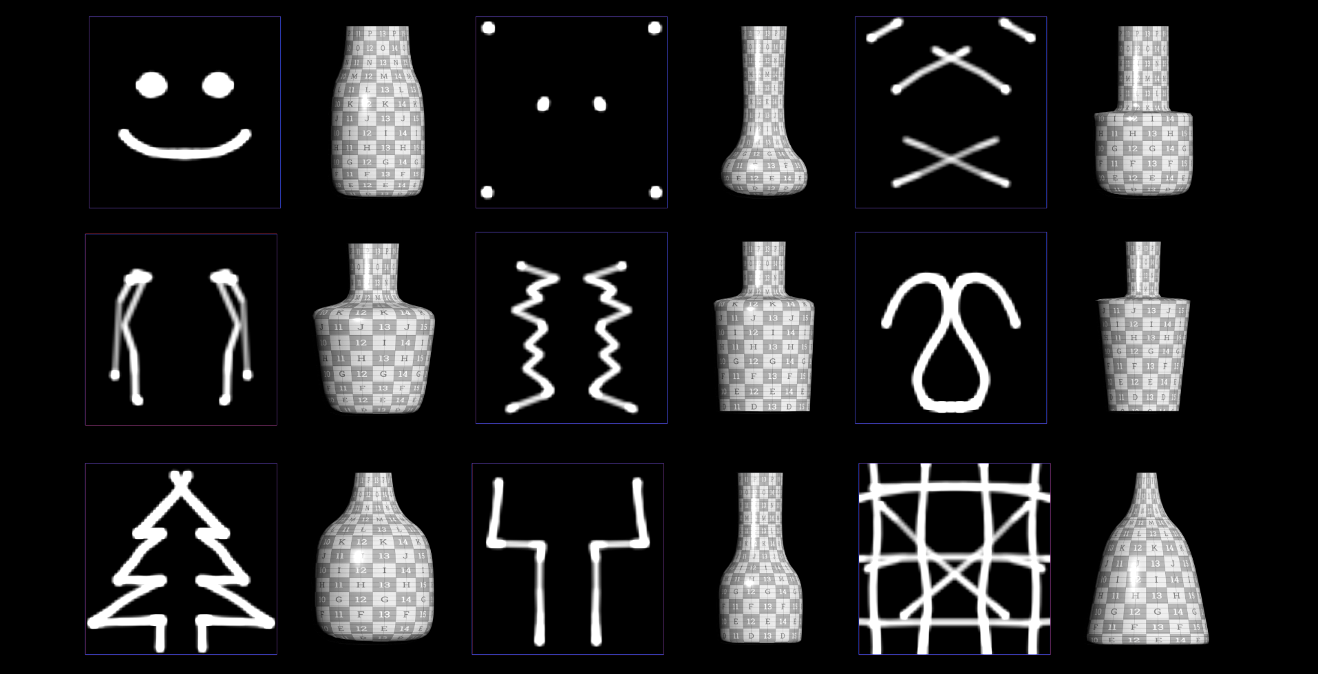
データの概要
下図は、ここまで用意したデータの全てです。
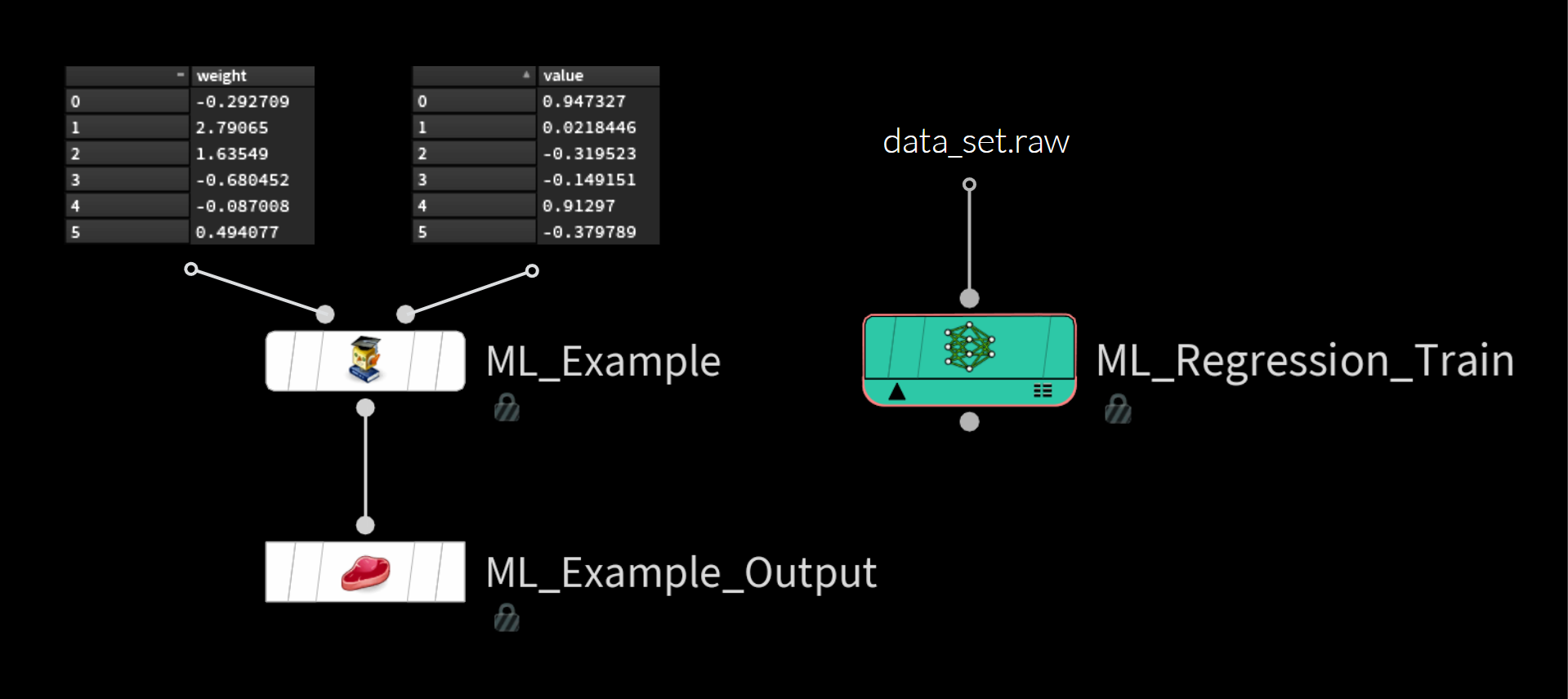
訓練サンプルを構成している値はわずか2つです。
- 入力: PCA サブ空間で瓶の輪郭の絵を描くウェイト
- ターゲット: ボトルの形を記述するパラメータ値
ML Examples Output SOP を使ってこれらの値を data_set.raw 形式でディスクに保存し、その後、 ML Regression Train TOP 内に読み込んでいます。
訓練
データセットを準備し、その .raw ファイルをディスクに保存したら、残りはごく簡単です。
特に重要なものは以下の通りです。
- Uniform Hidden Layers (ネットワークの幅の大きさ)
- Uniform Hidden Width (各レイヤに含まれる「ニューロン」の数)
- Batch Size (平均を取りウェイトを調整する前に見るべきサンプルの数)
- Learning Rate (ゴールまでにモデルが取るステップの大きさ/山から飛び下りるか、慎重に歩いて下るかの違いのようなもの)
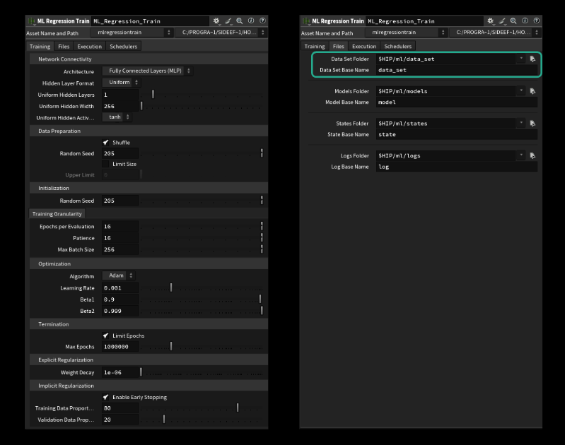
Files タブで適切な辞書とデータセット名を指定すれば訓練を開始できますが、デフォルトで正しい設定になっているはずです。注意 : ファイル名を指定する際、拡張子を付けないでください。「.raw」を付けると実行されません (H20.5.370 で最終確認)。
あとは、TOPノードをクックするだけで、うまくいけば思い通りの結果が得られ、十分な訓練データを取得することができます。
推論
TOPs 内のノード上に全てのパラメータが揃っているので、そこで最適化をしていきます。これは、ハイパーパラメータチューニングと呼ばれる一般的な手順で、何度か実験を繰り返し、最も性能の良いモデルを返す最適なパラメータの組み合わせを見つけます。先述のパラメータから最適化を始めるのが良いでしょう。ここで使用したグルームの変形サンプルでは、レイヤの量および各レイヤのサイズに関する最適化のみを行いました。
例によって、入力から正しいシェイプを得るには、データ生成の全工程を実行せねばなりません。そのため、確実に左右対称になるよう画像をミラーリングしてユーザ側でエラーを回避し、その後、新しい Mono to SDF COP ノードで、それを変換します。PCA にそれらのウェイトをサブ空間に投影させ、入力のウェイトを計算させます。
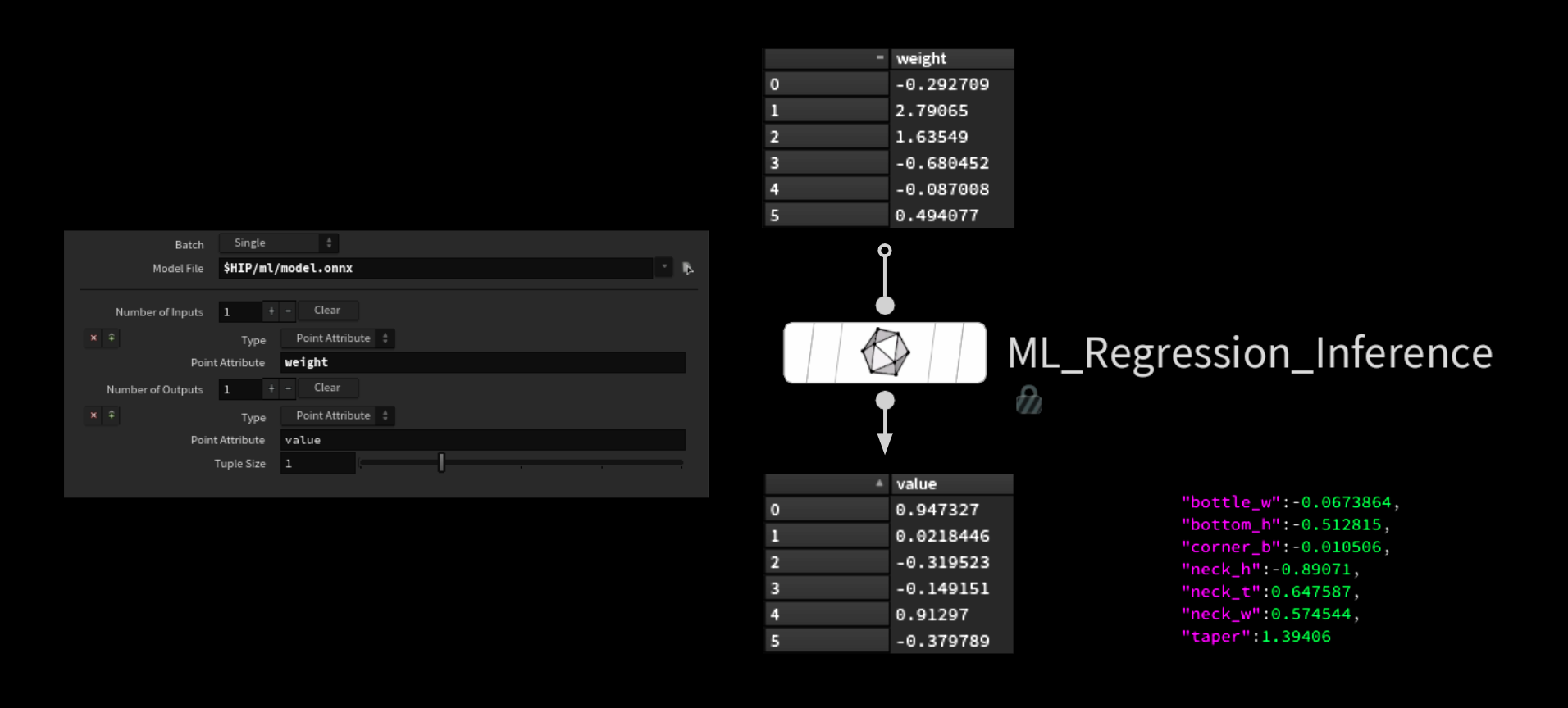
その後、それらのウェイトを選び、ML Inference SOP ノードに流し込み、作成したモデルに適切なパラメータを推測させます。
得られた値のリストを辞書に変換し、ジェネレータに送ります。このジェネレータがボトルのジオメトリを作ります。
パフォーマンス
推論の工程はとてもスピーディでリアルタイムで実行されます。ここでボトルネックとなるのはジオメトリ生成の工程です。単純なボトルではなく船の構築など、ごく複雑なHDA にシステムを繋ぐ場合、パフォーマンスの問題が生じます。その場合、以下の 2種類のHDAを用意すると有効な場合があります。
1. シルエット生成と大まかなシェイプを手早くイテレートするための HDA
2. 低解像度のドローイング用キャンバスでは捉えられないディテールの追加や形の微調整のための HDA
COPs
それを、いくつかのプロシージャルな COPs テクスチャセットアップと組み合わせれば、実際よりずっと複雑な見た目の結果を得られます。
出典 (テクスチャセットアップの作成): Dixi Wen
制約
同僚に見せたところすぐに、ランダムなシェイプを描き始めましたが、そのようなシェイプは、アーキテクチャの制約上、ジェネレータでは生成できません。
これは、欠点でもあれば利点でもあります。入力が何であれ常に合理的な結果が返ってくる一方で、ジェネレータで何が作成できるかによって出力内容が制限されます。
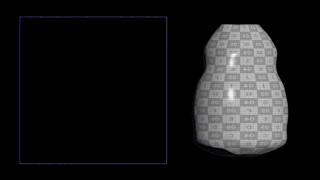
フル SDF を予測させてみる
PCA は SDF の圧縮において非常に有効なのは先ほど見た通りですが、パラメータではなくフル 3D の SDF を予測させるとどうなるでしょうか。
先ほどと同様、PCA に入力を圧縮させますが、ここでは出力にも圧縮を実行します。
3D による再構築は Fog ボリューム状の見た目です。
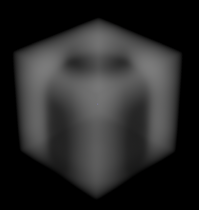
それを変換して VDB のメッシュ化テクニックで少しクリーニングアップし、UV 処理済みのクリーンなジオメトリをそこに投影すると、ボトルを得られます。
2つのジェネレータを用意する
この手法の主な欠点はジェネレータが2つ必要になることです。ひとつは訓練データの生成用で、もうひとつは、優良なトポロジと UV を持つ使用可能なジオメトリに SDF を変換するためのものです。これは最大の難点でもあります。ボトルは最も簡単なシェイプのひとつですが、あらゆるオブジェクトが簡単に優良なトポロジに変換できるわけではありません。
左が訓練データの生成で使用するオリジナルのジェネレータです。パラメータの値をターゲットとして格納する代わりに、ボトルのジオメトリに由来するフォグの SDF を格納しています。
推論
入力に対しては、先ほどと同じ作業(ミラーリング、SDF への変換、PCA による投影)を行います。その後、PCA を使って出力を実行し、予測したウェイトを元に、3D SDF を再構築します。この SDF をふたつめのジェネレータに流し込んでクリーンなジオメトリに変換します。
パフォーマンス
精度と柔軟性は向上していますが、生成速度には難があります。
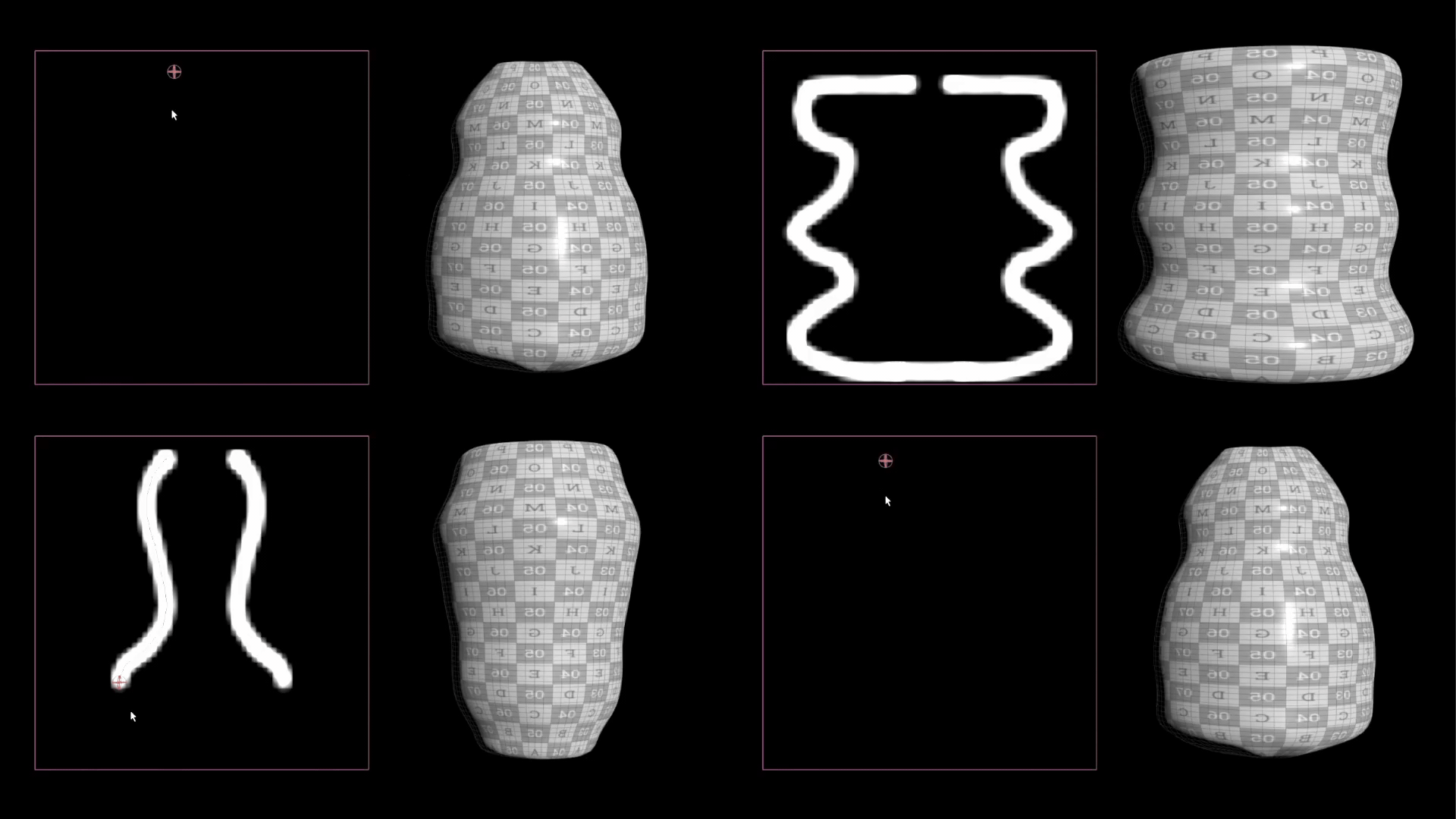
ふたつめのジェネレータがボトルネックとなったことで、先ほどと比べると速度が格段に落ちました。ただし、出力内容の柔軟性がはるかに高く、訓練データには存在すらしない「中間」シェイプも描くことができます。急カーブや出っ張りができてしまうといった問題も残っており、これはその他の技法やより優れた訓練データによる改善の余地があります。
謝辞
このプロジェクトを支えてくれた、SideFX の優秀なチームの皆さんに感謝します。
全面的なサポート: Fianna Wong
ML ツール開発: Michiel Hagedoorn
COPs のボトルのテクスチャセットアップ: Dixi Wen
CREATED BY

コメント
aparajitindia 1 ヶ月, 4 週間 前 |
bravo. Absolute explode on explanation. Sir so much to understand. Thanks for brain storming.
Aparajit from India.
Masoud 1 ヶ月, 4 週間 前 |
It's amazing, thank you very much.
freelancerakash11 1 ヶ月, 3 週間 前 |
It's amazing, thank you very much.
mzjorxd 1 ヶ月, 3 週間 前 |
It's amazing, thank you very much.
I would also like you to develop a real-time interaction tool between ComfyUI and Houdini, so that the early planning and communication phase will be very convenient
Please log in to leave a comment.