The new MPM solver in Houdini 20.5 enables us to achieve an incredible organic crumbling feature in a fairly straight forward setup. In the next few chapters I am breaking down each step to create the snowplow scene in the Houdini 20.5 sneak peak.
Before we start, keep in mind that MPM simulation can be very memory intensive, the final high quality caches for this project was around 2 TB. The project was done in Windows 10, RTX 3090 (555.99) , AMD Ryzen Threadripper 2970WX 24 Core Processor and 128gb ram.
Step 01 - Prepping materials
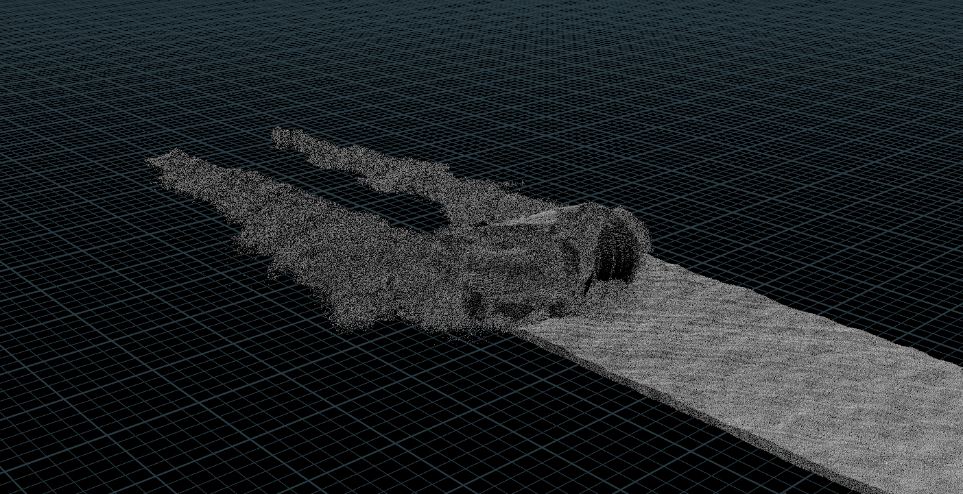
The idea for this project is to really focus on the snow details; my goal was to see chunks of snow rolling on the floor while they crumble and get broken down.
Starting from getting all the ingredients ready, preparing models for collision is very straightforward:
I’m using a very nice plow model, to which I will simply add some movement noise and the characteristic angle offset. Once we are happy with the movement, we are left with some research on what’s the average snow plow speed and try to mimic it inside of our scene with a follow path node.
Drop an mpmcollider node → Set the collision type(Animated Rigid) → Use Input Animation → Done.
Inside the mpmcollider there are a couple of options to adjust according to your collision type, these are:
Collider Type
Use Input Animation
Geometry Tab → Custom Voxel Size and Fill Interior
Repeat the whole process for the rest of your collision and keep an eye on setting the correct Collider Type.
Once the collisions are ready, let’s have a look at mpmcontainer and mpmsolver. After this we can focus on sourcing the actual snow.
Step 02 - MPM Container and Solver
MPMcontainer is the “mastermind” node for all the setup, from there you can control the simulation, sourcing, collision voxel size (“resolution”), time step and frame start. There are other attributes, such as Grid Scale that for this setup are perfect at the default value. This can be useful when you are simulating with multiple materials to avoid material from sticking to each other.
Step 03 - MPM Material Sourcing
Import your surface and drop a mpm source node and choose Snow as Material Preset with Chunky as Behaviour. These recipes are well balanced for each material, so there is no need to go far away from those values.
That said, let’s try to get far away from these values.
To achieve variance some variables to keep in mind are:
Stiffness, represented as E (@E).
Density, represented as Density (@density).
Volume Preservation, represented as Nu (@nu).
In this scene I want to have some ice blocks and fresh powder, as if this piece of snow was freshly compacted.
Stiffness is your go-to while trying to hit a better performance/result ratio. Having higher stiffness in the center will play a crucial role in keeping the material malleability properties. Left image has a stiffness of 0, while the right example will have a denser core (x10²) and slowly fade to the material preset value.
It’s important to reference real Materials Density and iterate with smaller particle count. In my case. I can say that while Ice and fresh snow sits between 300 to 917 kg/m3 I can confidently insert variations ranging from 400 to 860, knowing that I will still retain some nice chunky details and at the same time, some powder clumps. *you can find these sources at the bottom of the page*
These noises are meant to introduce variation and “help” the material fracture following a specific art direction, it’s important to keep in mind that MPM strengths reside in mimicking how forces act, resulting in breaking the materials organically.
The very fine dust will be done later in a secondary pop simulation.
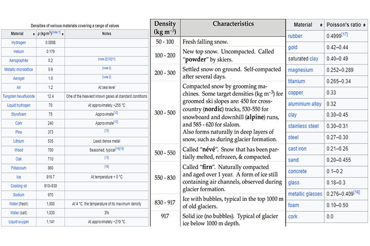
Volume Preservation is how much perpendicular force a material should have under any given compression, this is also known as Poisson’s Ratio in solid mechanics. Also for this, there are plenty of good references about each material’s Poisson’s Ratio. These values are a great starting point, wedging this simulation at a lower point count is key to get the right feel and look.
-In simple words this value is very sensitive, the higher the volume the more force is propagated, the lower the more force is dissipated through out the material-
Here are some tests with different values with : 7M points, and then upscaled to 24M points.

Note
Consider the area you want to convert, MPM simulation can easily sit around 80 Million Points, with each of them storing attributes that can be very helpful later on. Be mindful of what you use and need and always remove attributes that are not needed.
Simulate at lower resolution and when you feel there is a little bit of structure, try to send a higher quality simulation overnight ( 20 Million pts already will give you the final look idea ).
To achieve a specific look, take into consideration the thickness of your starting mesh and the stickiness of different surfaces ( it’s a slider, not on/off ).
The more material you use, the more vram will be needed to store all the attributes needed; before sending off the final simulation, calculate how much you can push it to avoid mid frame crashes ( Usually when particles get shot off increasing the VDB grid size).
Understand what sort of scale you need before starting the simulation using the point size, Default is at 2. It would work fine up to a mid range, the closer you get, the more points you will need.
Keep it simple.
For best results, use materials table as a reference point.
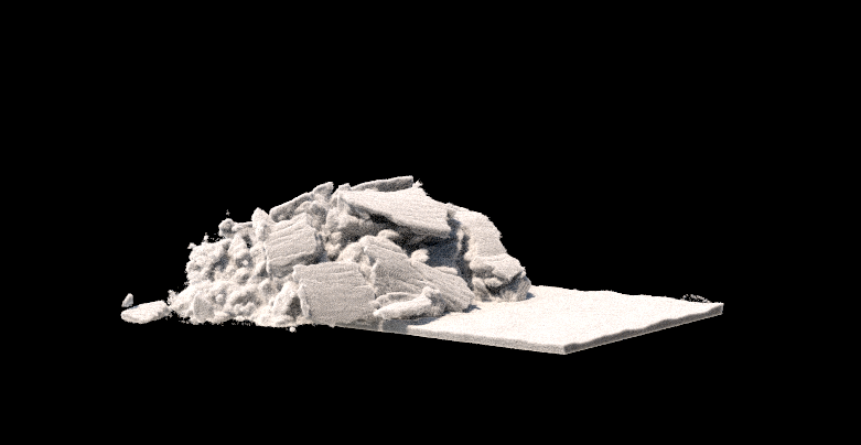
Step 04 - Post Sim Meshing
Post simulation is where the MPM setup starts to get more articulated. It’s expected to have a very grainy look.
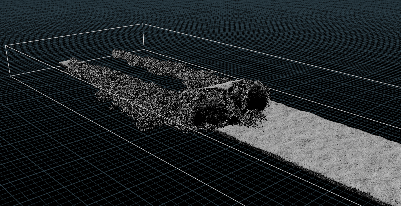
In this setup, the best solution is to run the points through a VDB block (particlefluidsurface does the same passage):
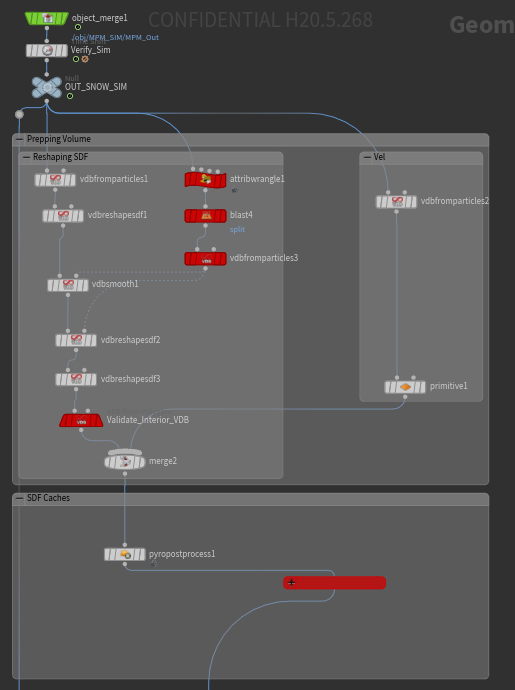
Here I can convert the MPM particles using @dx detail attribute as my voxel Size. I will convert them to SDF and there take advantage of vdbreshapesdf to really art direct the look of my volume; in this case, I’m doing Dilate → Smooth → Erode (only the outer edges) → Erode the same amount I dilated.
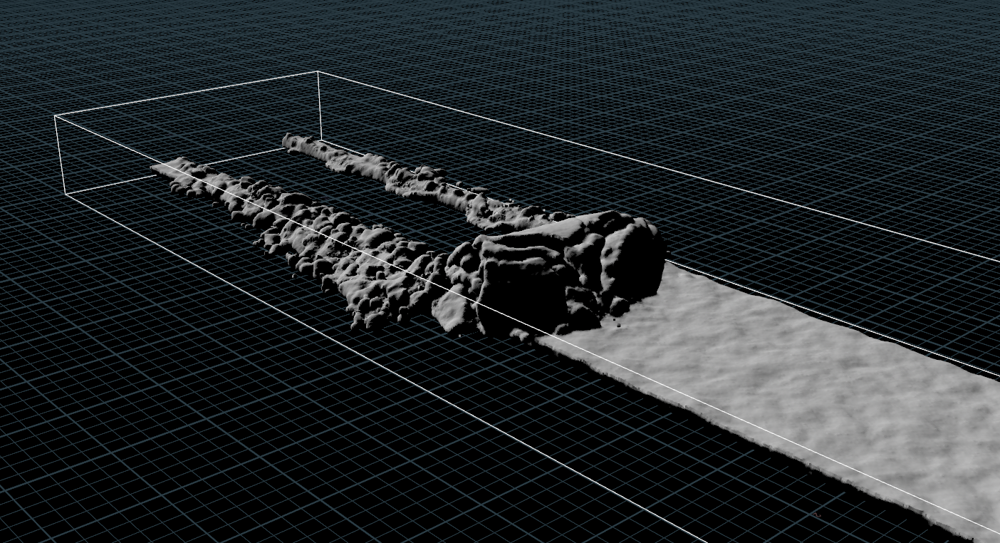
The result looks like this:
After we achieve a look we are happy with, let's merge it with a velocity field and cache the SDF volume. -this will be useful later on to achieve a good collision source for the secondary simulation-
To retain more quality, I noticed that balancing the voxel sizes and particle scale really plays a big role. It’s good to start looking for the final output early on.
After rasterizing the main MPM sim with a VDB grid, we can now clamp this volume with the reshaped SDF volume, and push toward sharpening it before the volume starts to show artifacts.
This part can play a major role in the final look, you can extract more details than the main sim has, but be prepared to see floating elements and other artifacts. On the other hand, you can dial this back having a more cohesive look, sacrificing the very sharp high details.
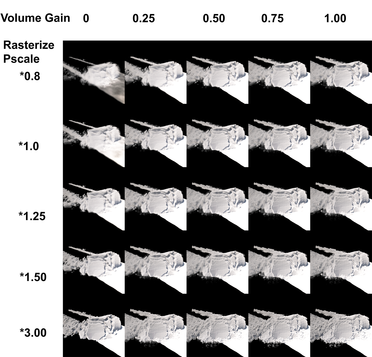
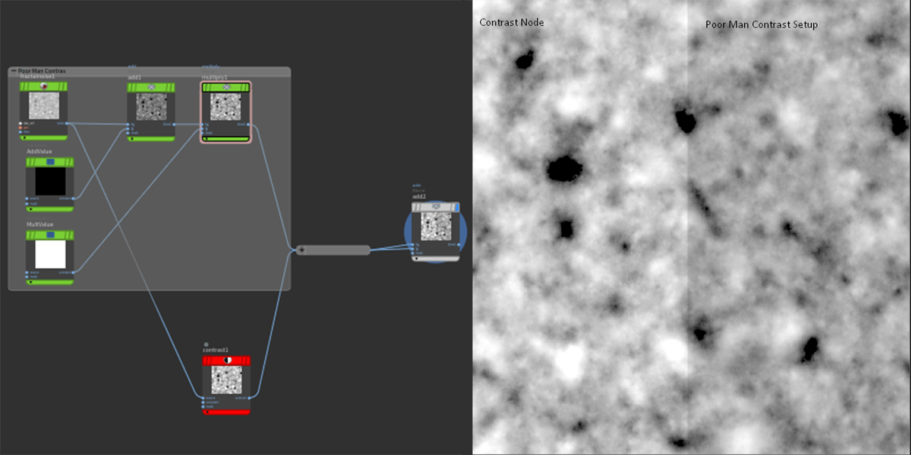
Another trick that can be helpful is to manipulate it like you would do with an image, gain and contrast, and the result gets clamped with the SDF again. We are trying to achieve the sharpest look without introducing floating particles or fuzziness in the final render. If you want to see the results without waiting for render, you can simulate this in the new COP Network.
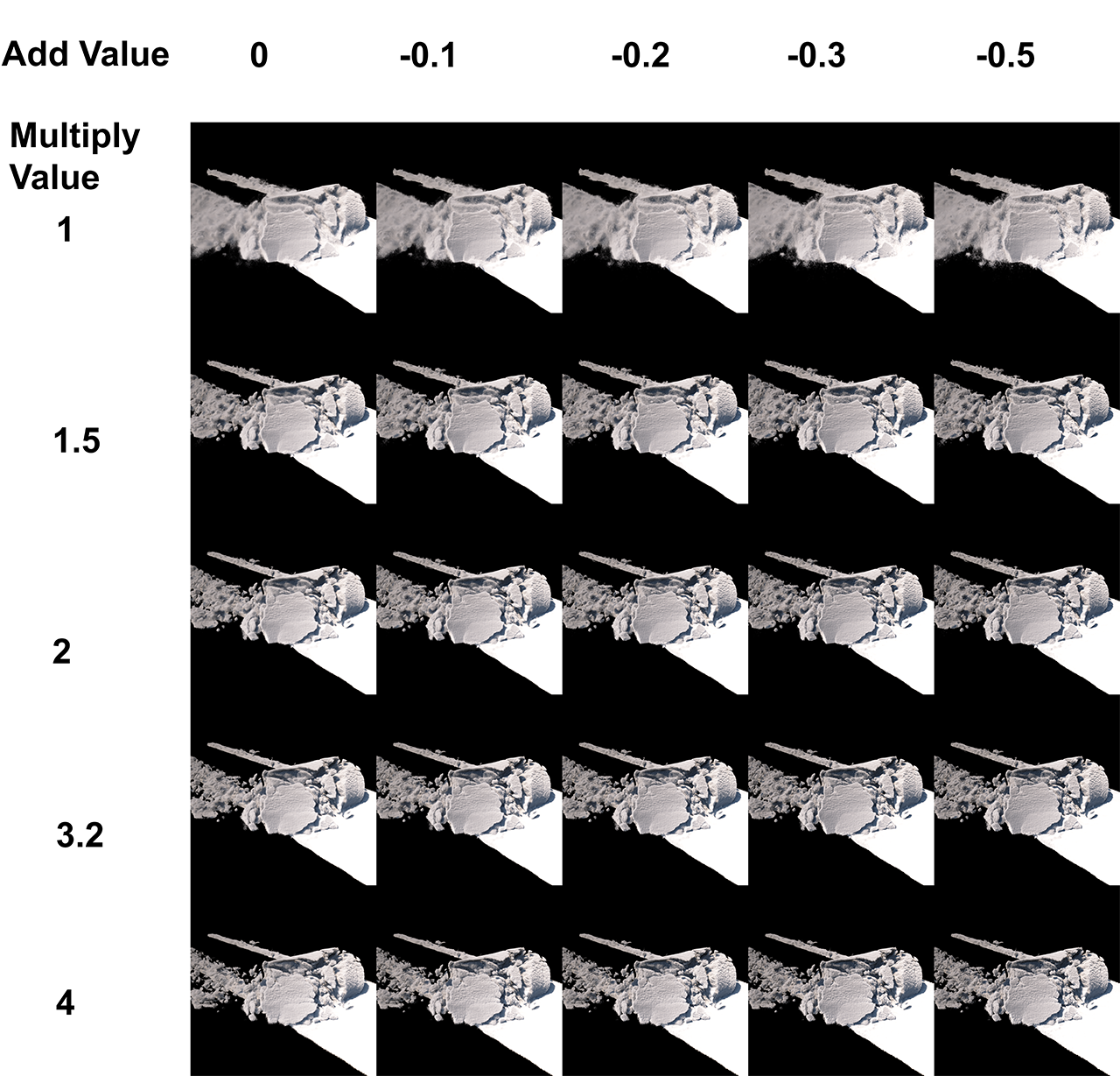
Using a contrast node plugged after a noise fractal, we achieve a sharpening effect, but if we subtract values and then multiply the result - we achieve the same results and this can also be easily applied to volume fields!
Here is an example with different values:
At this point, you should be happy with the result, we can still fine tune it afterward in LOPs.
Note
Meshing MPM can be tedious, work on small batches and once you are happy with it, apply it to the full sim.
Try to block a final material early on and iterate with that one.
Keep in mind that the sharper you get, the more floating volumes there will be; the key is patience in finding the good spot.
Double Check if your SDF volume is filled inside, if not, you might need to validate it to avoid issues during secondary pass.
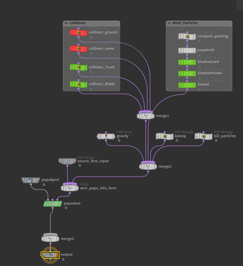
Step 05 - Secondaries setup
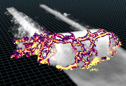
Secondaries play a big role in snow scenes, this is why planning ahead is key. Our main attribute will be @Jp . JP represents the critical stress, areas of the materials that are breaking, or under stress, while maintaining lower value for particles that are resting.
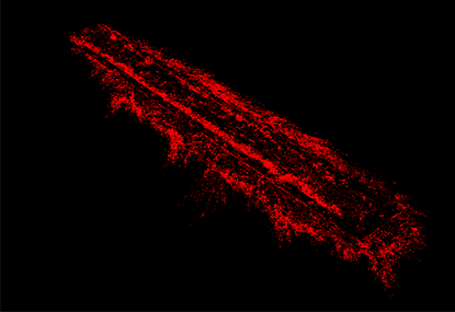
Starting from sourcing the correct points from the attribute, I decided to filter the main mpm source calculating the difference between JP Values and isolating it from the source (¹) then pushing it forward to help the sim get the right feeling. Another element I wanted to introduce was generating a cluster of particles when a big chunk of snow hit the floor. (²) After which I merged all the source points and verified that none of those were within the collision surface, to avoid weird shooting particles.
Collisions element: Main Ground, MPM SDF (that we cleverly cached before ;-) ), Collision Truck and Collision Blade.
-this can be done also using static objects-
Wind Particles: It will add air drag based on particle packing; useful to simulate this sort of particle effect, then the shadow elements.
The rest is the standard POP setup, I just added an asleep line to optimize the scene as much as I could and a Kill threshold under the ground, in case some particles fell through.
The meshing process is the same as before. Just rasterize the particles by 0.8/1.2 of the particle pscale and contrast the noise to get a sharper feature. Here too - patience is key, isolate one frame and portion with high movement and work from there.
Note
Also in this case, the particle count can easily go to very high numbers. In my case, I found a good balance within 10 Million particles at the end of the sequence.
Before we proceed to launch the simulation overnight, it’s worth it to verify what the correct @pscale you need in function to your camera angle, in my case it was 0.0012. Also visualizing it using discs can help dramatically
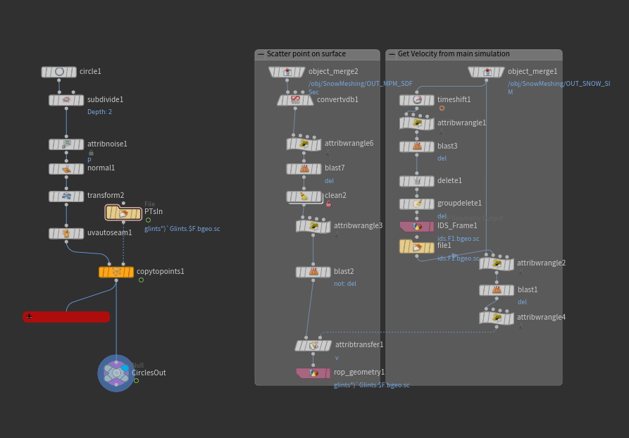
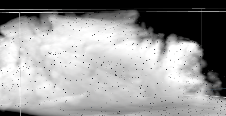
Step 06 - Snow Glints
The next step is not fundamental. At some point, there will be details that are not visible from the camera angle/lighting and movement, this can be glints.
A few things I wanted to keep in mind, glints needed to be randomly generated on the surface of the volume since it’s the little frozen droplets and I wanted to keep some of the original attributes from the original mpm simulation. Once we have points that are on the surface with the correct velocity value, we can proceed with a copy to point to scatter a disk on those points.
Note
- Test your glint sizes in a small portion of the simulation, sometimes you need to double check with the render fog volume to make sure it will sit on the surface.
- Your best friend in this case is blast node for the points and VDB clip for the volume.
- If you add a notch of noise to the disk, you might be able to have more interesting results.
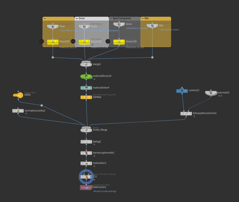
Step 07 - Rendering in Solaris
The render setup is a standard tree. The only element to consider is to give more attention to the materials for the snow body and the glints.
Glints must be a transparent material with high specularity, while for the snow, we take advantage of Material Linker and assign a quick cloud material to our volume and add or remove density according to the look you are looking for.
Note
For the final look, take advantage of the different AOVs available and leverage an optix denoiser with a volume combine pass to achieve a good organic texture, while keeping the render as clean as possible.
While doing look dev, it’s best to avoid using denoiser, since a lot of details in the snow will get wiped out in the first few samples.
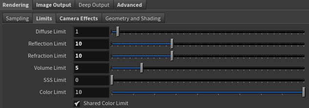
Don’t forget to increase your volume limits.
Wikipedia.com - List of Materials Density (Site:” https://en.wikipedia.org/wiki/Density#Various_materials “ Accessed: 06.17.2024 )
eoas.ubc.ca - List of Fresh Fallen Snow Density (Site: “ https://www.eoas.ubc.ca/courses/atsc113/snow/met_concepts/07-met_concepts/07b-newly-fallen-snow-density/ “ Accessed: 06.17.2024 )
CREATED BY

COMMENTS
ostaek 8 months ago |
Thank you very much for the in depth tutorial and explanation! So much valuable insights and lesson. I was wondering if we can get the COP workflow in the hip file too
aparajitindia 6 months, 1 week ago |
thank you. i am in the learning process. great help to understand.
love from india
aparajit
9405587742
pixolator 4 weeks, 1 day ago |
Thank you very much !
Please log in to leave a comment.