The Copernicus network uses and refers to the following spaces:

• Buffer: The samples of the image, which correspond to the data layout in the memory.

• Pixel: A canonical pixel-sized area. The pixel’s origin coordinates are the lower-left corner of the pixel. The display window determines the image’s location in this pixel array. The data window determines the Buffer’s location.

• Texture: Maps from 0 through 1 across the data window and Buffer space, which stretches the texture.

• Image: Maps from -1 through 1 across the display window, which scales the image to fit to preserve the pixel aspect ratio.

  Note

  The preview thumbnail for a COP node displays the output in a -1 to 1 window.

• World: A 3D location in the modelling space. For example, the viewport applies this space when you use a Transform 3D COP.

Instead of always using texture space, Copernicus uses image space. Since Copernicus is linear first, it can use negative values. This means Copernicus values are in their natural space (a requirement for HDR) instead of being normalized. The following are additional benefits of keeping values in their original space:

• You don’t need metadata that indicates the value’s actual range.

• Ranges aren’t clamped . This means HDR, vectors, and such aren’t limited.

• The values are one-to-one with the SOP version of attribtues.

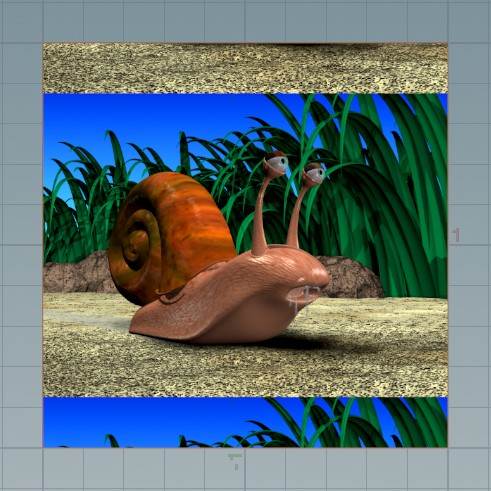
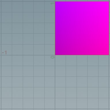
The 3D viewport imports Copernicus nodes using world space, which by default is the same as image space. This frames the image in a -1 to 1 square, which creates borders for non-square images since their coordinates cover only some of the -1 to 1 range. In comparison, the texture space always covers the 0 to 1 range for the image data.

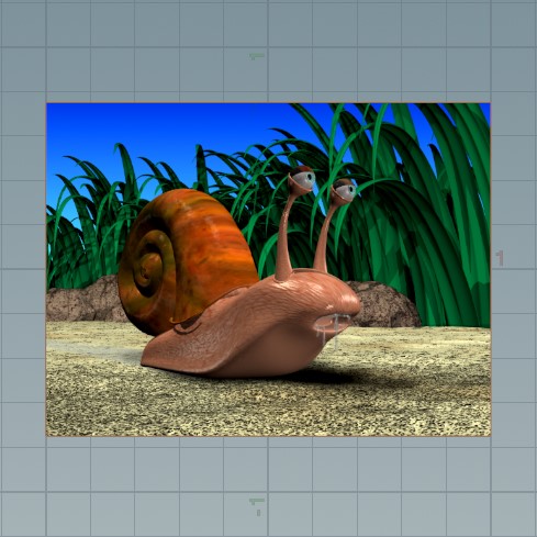
Comparison of a square and non-square in image space.

Cropping ¶

When you Crop in image space (set Units to Image), the default crops from -1 to 1. This makes a non-square image bleed outside of texture space to fill the image space. An image space crop is an absolute crop. For example, if you wire in two identical Crop nodes where Lower Left is 0, 0 and Upper Right is 1, 1, the final output is a quarter of the original image since the values of the two Crop nodes aren’t applied on top of each other.

When you Crop in texture space (set Units to Texture), the node crops the image based on the incoming image’s data window. This prevents a non-square image from bleeding outside of texture space. A texture space crop is a relative crop. For example, if you wire in two identical Crop nodes where Lower Left is 0.5, 0.5 and Upper Right is 1, 1, the final output is a sixteenth of the original image since the values of the two Crop nodes are applied on top of each other.

Note

The image doesn’t move in the viewport when you adjust the Crop settings if it’s in texture space and the Crop node’s Mode is set to Discard Cropped. For information about how to change this setting and reframe the cropped image, see the Crop COP’s Mode parameter settings.

When you Crop in pixel space (set Units to Pixels), the node crops the image based on the exact pixel values you set in the node.

Visualization ¶

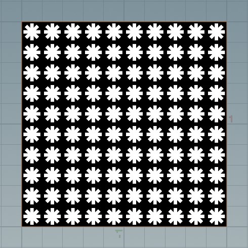
Visualizing refers to when you perform UV mapping in the viewport instead of displaying the real colors of an image.

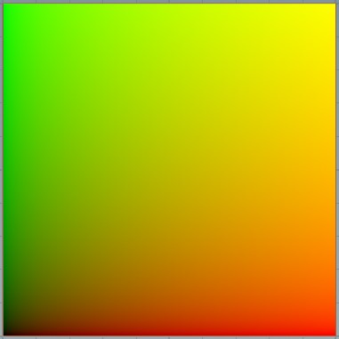
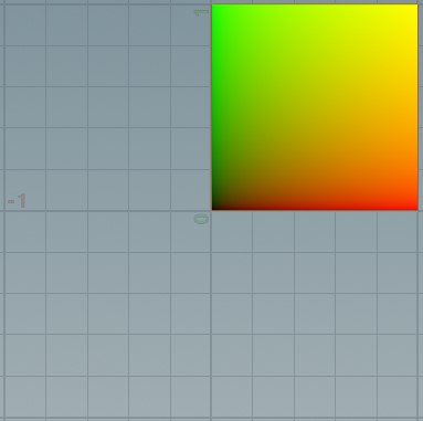
When you wire a Crop node into a UV Map that has UV Space set to Image, the output displays the remaining section in the color that originally occupied the section.

Comparison of original and cropped UV image space.

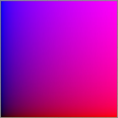
When you wire a Crop node into a UV Map that has UV Space set to Texture, the output displays the remaining section in the entire color gradient of the original image.

Comparison of original and cropped UV texture space.