| On this page |
The ![]() Houdini Procedural: RBD LOP is an alternative to the
Houdini Procedural: RBD LOP is an alternative to the ![]() RBD Destruction LOP that gives you full control over the import process. If you still want to use the destruction node as higher level tool, you can do that. There you also have access to the procedural when you set Output Type to`Procedural. However, the new procedural is the recommended replacement for the destruction LOP’s other Output Type modes like Deforming Mesh or Dynamic Skinning.
RBD Destruction LOP that gives you full control over the import process. If you still want to use the destruction node as higher level tool, you can do that. There you also have access to the procedural when you set Output Type to`Procedural. However, the new procedural is the recommended replacement for the destruction LOP’s other Output Type modes like Deforming Mesh or Dynamic Skinning.
The idea behind the procedural method is that users often had issues with bigger scenes at production scale. For example, large amounts of fractured pieces created an appropriate number of primitives - either as prototypes or individual objects. This normally lead to performance and naming problems, and the scene required (much) more disk space.
The Houdini Procedural: RBD is a separate tool that wraps up workflows from RBD/simulations and the USD side to solve the aforementioned issues. With the new tool, the USD stage remains manageable and shows only the original primitives in the Scene Graph Tree.
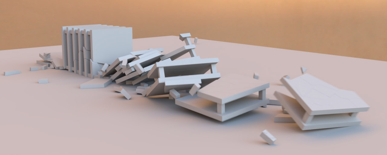
The following chapters illustrate how to use the new procedural in conjunction with a typical destruction scene: a tower-like construction falls down on a ground and breaks apart. The workflow scene is just an example, and you can use other objects as well.
Note
All workflows, described on this page, assume that Houdini’s Solaris desktop is active. You can find this desktop in the main menu bar’s first dropdown menu (the default desktop is Build).
SOP setups 
One big advantage with the new procedural is that all SOP workflows are still the same and you set up your RBD scene in the exact same way as before.
-
In this example, an
 RBD Material Fracture SOP breaks a tower into individual pieces.
 -
The
 RBD Bullet Solver SOP performs the simulation.
Outputs and caching 
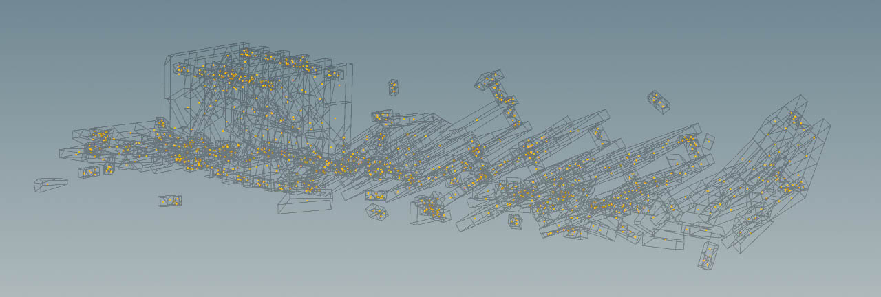
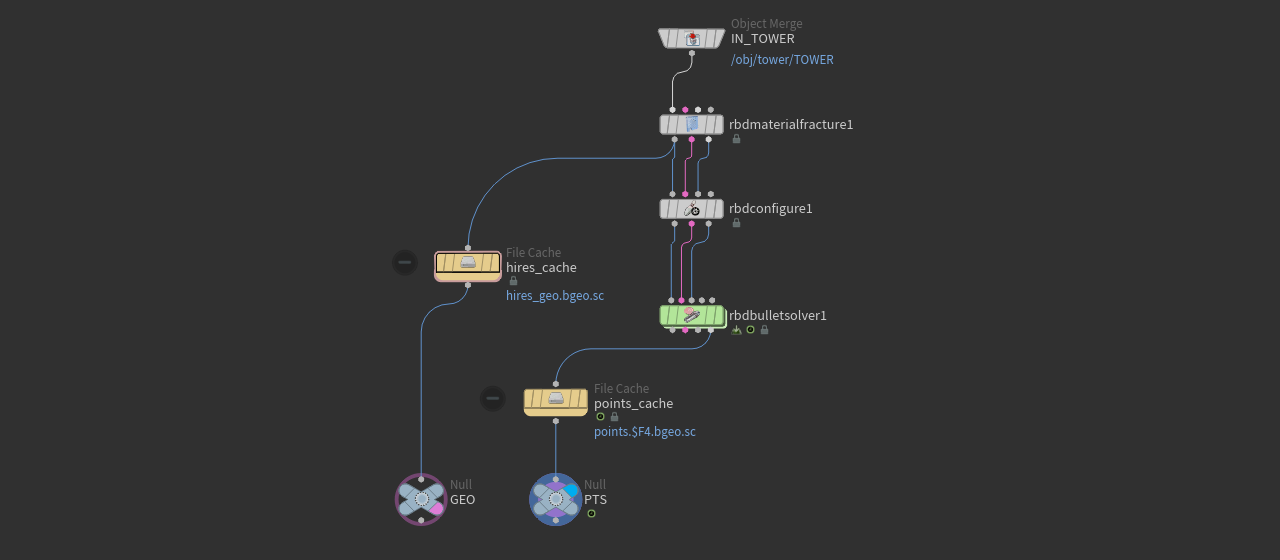
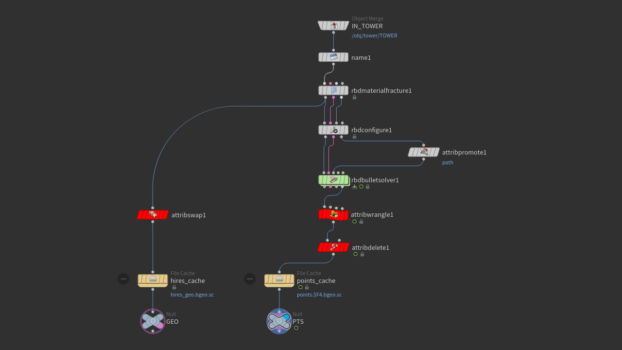
The solver’s outputs contain the original high-resolution geometry, the constraints, a proxy version of the object and the fracture points. The last output is of particular importance: the points carry the necessary motion information from the simulation and you can use them to drive the pieces as shown in the image below. So, you only save a couple of points over the entire simulation range. This is much more resource-friendly than saving of hundreds or thousands of individual objects. To connect pieces and points in the procedural, you also need the one copy of the fractured high-resolution geometry.
-
Add a
 File Cache SOP and connect its input with the first output of the RBD Material Fracture SOP. Make sure to create a separate branch for the file cache node. Rename the node to
 hires_cache. -
Turn off Time Dependent Cache to save only one copy.
-
If necessary, adjust Base Name and Base Folder to your needs.
-
Click Save to Disk to write the geometry to disk.
-
Lay down another File Cache SOP. This time, connect its input with the fourth output of the RBD Bullet Solver SOP. Rename the node to
points_cache -
Again, set name and folder if you need it.
-
Then click Save to Disk or Save to Disk in Background to cache the simulation range to disk.
Now that you have all data on disk, you can finally add a ![]() Transform Pieces SOP to bring everything together again. Connect the output of the first file cache to the transform’s first input; the points go to the second input. The Transform Pieces SOP isn’t relevant for the procedural and only for previewing the simulation.
Transform Pieces SOP to bring everything together again. Connect the output of the first file cache to the transform’s first input; the points go to the second input. The Transform Pieces SOP isn’t relevant for the procedural and only for previewing the simulation.
Nulls 
In Houdini it’s very common to terminate network streams with ![]() Null SOPs. The SOP setup for the RBD procedural is no exception and here the Nulls will carry all the necessary information for the simulation.
Null SOPs. The SOP setup for the RBD procedural is no exception and here the Nulls will carry all the necessary information for the simulation.
-
Add a Null SOP and connect its input with the output of the
hires_cacheFile SOP. Rename the node toGEO. -
Lay down another Null SOP. This time connect its input with the output of the
points_cache. Rename the node toPTS.
path attribute 
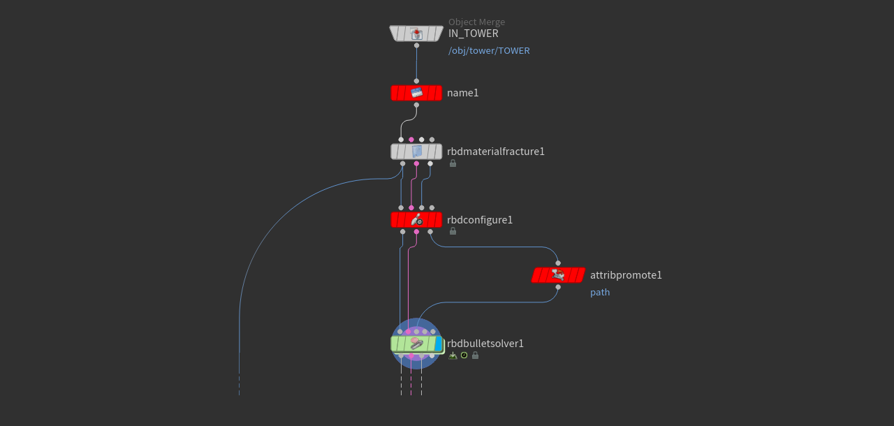
Names and paths are essential in conjunction with the RBD procedural. Everything begins with a path. A path attribute controls how the geometry is partitioned into USD primitives: you’ll avoid to create one Mesh primitive per piece. The attribute will therefore improve scalability for the procedural in conjunction with large amounts of pieces. And then you also need a separate attribute to identify the pieces within those Mesh prims that contain multiple pieces.
Looping the path attribute through the RBD simulation requires several steps and here you have to be very careful: if you're missing just one step, the procedural won’t be able to connect points and pieces.
Tip
To keep track of the various attributes, open the Geometry Spreadsheet pane. You can toggle between point and primitive attributes with the ![]() and
and ![]() buttons.
buttons.
-
Add a
 Name SOP to your network and connect its input with the output of the last node that creates your object. Depending on your scene, this can be, for example, a basic
  Sphere SOP, but also a
  Merge SOP. If your object comes from a different network, you most probably use an
  Object Merge SOP, etc.
Connect the name node’s output with the input of the first node of the RBD/fracture branch of your network, e.g. the RBD Material Fracture SOP.
-
For the name node’s Attribute, enter
path. -
Go to Name and enter something like
/scene/tower. This path will later appear in the Solaris Scene Graph Tree. Of course, you're free to change the path according to your own requirements. -
Lay down an
 RBD Configure SOP and connect the first three inputs with the appropriate outputs of the upstream RBD Material Fracture SOP. Then link the three outputs with the first three inputs of the RBD Bullet Solver SOP.
 -
On the Attributes section, go to Transfer Attributes and append
pathto the already existing attributes. -
Add an
 Attribute Promote SOP and connect its input with the third output of the RBD Configure SOP. Link the output to the third input of the solver.
 -
For Original Name, again enter
path. -
Then, open the Original Class dropdown menu. Choose Primitive to transfer the
pathattribute to the (simulation) points. -
Finally, select the RBD Bullet Solver SOP and open the Output tab. Go to Attribute Transfer and append
pathto the already existing attributes.
name and piecename attributes 
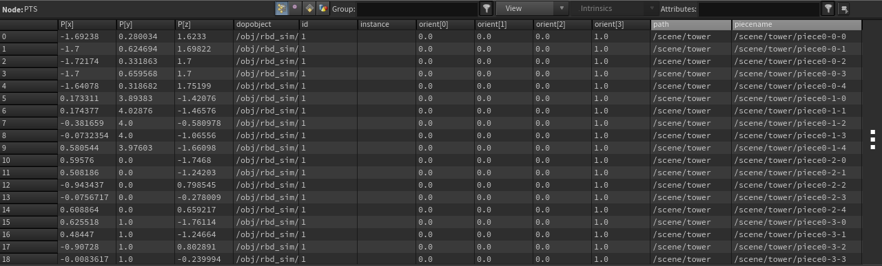
The RBD Material Fracture SOP automatically creates a name attribute to identify the individual pieces. When you look at the Geometry Spreadsheet in Points mode, you’ll see entries like piece0-0-0, piece0-0,1 and so on.
The name and path attributes, however, are also used internally by the ![]() SOP Import LOP in Solaris, so they won’t be available as primvars (primvars is how attributes are called in USD/Solaris) on the Mesh primitives. Therefore, it’s necessary to convert
SOP Import LOP in Solaris, so they won’t be available as primvars (primvars is how attributes are called in USD/Solaris) on the Mesh primitives. Therefore, it’s necessary to convert name into something different. A good choice is piecename, because it’s already the procedural’s default entry.
There’s also a good reason to delete the name attribute before you export everything to Solaris: the attribute is rather heavy.
Here’s a preview of the complete SOP network followed by the workflow description for the nodes you need to create the piecename attribute.
-
Add an
 Attribute Swap SOP. To make it a part of the
 GEOnetwork branch, place it between the RBD Material Fracture SOP and thehires_cacheFile Cache SOP. The connection is then established automatically. -
Open the Method dropdown menu and choose Move. This method works like a renaming process.
-
Set Source to
nameand Destination topiecename.On the RBD branch of the network you now need a point-based counterpart for
piecename, so that pieces and points can find together in the procedural. -
Put down an
 Attribute Wrangle SOP and connect its first input with the fourth output of the solver. Link the node’s output with the input of the
 PTSNull SOP. -
For VEXpression, enter
s@piecename = s@path+"/"+s@name;This one-liner assembles a string
piecenameattribute from thepathandnameattributes, and puts a backslash between both. -
Finally, add an
 Attribute Delete SOP and place it between the wrangle and the
 PTSnull to connect its first input. -
On the Point Attributes parameter, enter
name. The attribute disappears from the Geometry Spreadsheet and you can seepiecenameinstead along withpath.
Solaris setups 
Now you have everything you need and you can switch to Houdini’s stage level for creating the procedural network. You’ll now also make use of the attributes you've created before. Below is the smallest possible network setup.

-
On the stage level, create a SOP Import LOP.
-
Next to SOP Path, click the
 button to open a floating operator chooser. There, navigate to the
 GEOnull in the SOP network. File caching is optional and the import also works with “on-the-fly” simulations that are cached to your computer’s memory. -
The RBD Primitives field contains the content of the
pathattribute you've created in the SOP network. In this example it’s/scene/tower. You can also see this entry in the Scene Graph Tree and drag it from there to the parameter’s input field. -
Turn Piece Attribute and leave the default
piecenameattribute.
Points Location: Primitive 
The standard choice of Points Location is Primitive. If you did not cache the simulation to disk, leave this mode.
-
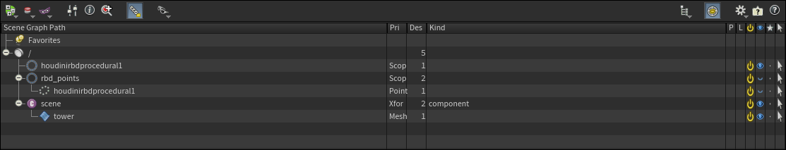
Point Primitive creates an entry in the Scene Graph Tree that will contain the simulation points from Points SOP. The entry takes name of the the SOP Import LOP (
$OS) to create a path. So, with the node’s default name, the path will be/rbd_points/houdinirbdprocedural1. Change this path to your needs. -
Next to Points SOP you can see an
Open floating operator chooser button. Click the button and use the tree menu to navigate to the PTSNull SOP. Click Accept to confirm your choice.
The Scene Graph Tree shows the Solaris hierarchy for the procedural
Points Location: File Cache 
When you change Points Location to File Cache, you can see a Points Cache parameter that lets you choose a file sequence with the simulation points from disk. If your file name doesn’t match the default pattern, click the ![]() Open floating file chooser button. Use the file browser to navigate to the folder with the files, choose the sequence, and click Accept.
Open floating file chooser button. Use the file browser to navigate to the folder with the files, choose the sequence, and click Accept.
Preview and render 
To see the result of your work, drag the timeline slider or press the ![]() Play button.
Play button.
The Houdini Procedural: RBD LOP has a Preview Procedural toggle that is turned on by default. This toggle lets you display the simulation in Houdini’s viewport and render it. If you, for whatever reason, don’t want to see the transformation, you can turn it off. Then, you’ll only see the rest state.
Note
Houdini’s procedurals work with any available render delegate.
To render the simulation, you don’t have to pay attention to anything special and you can perform the render process according to your specifications.