| On this page |
Introduction 
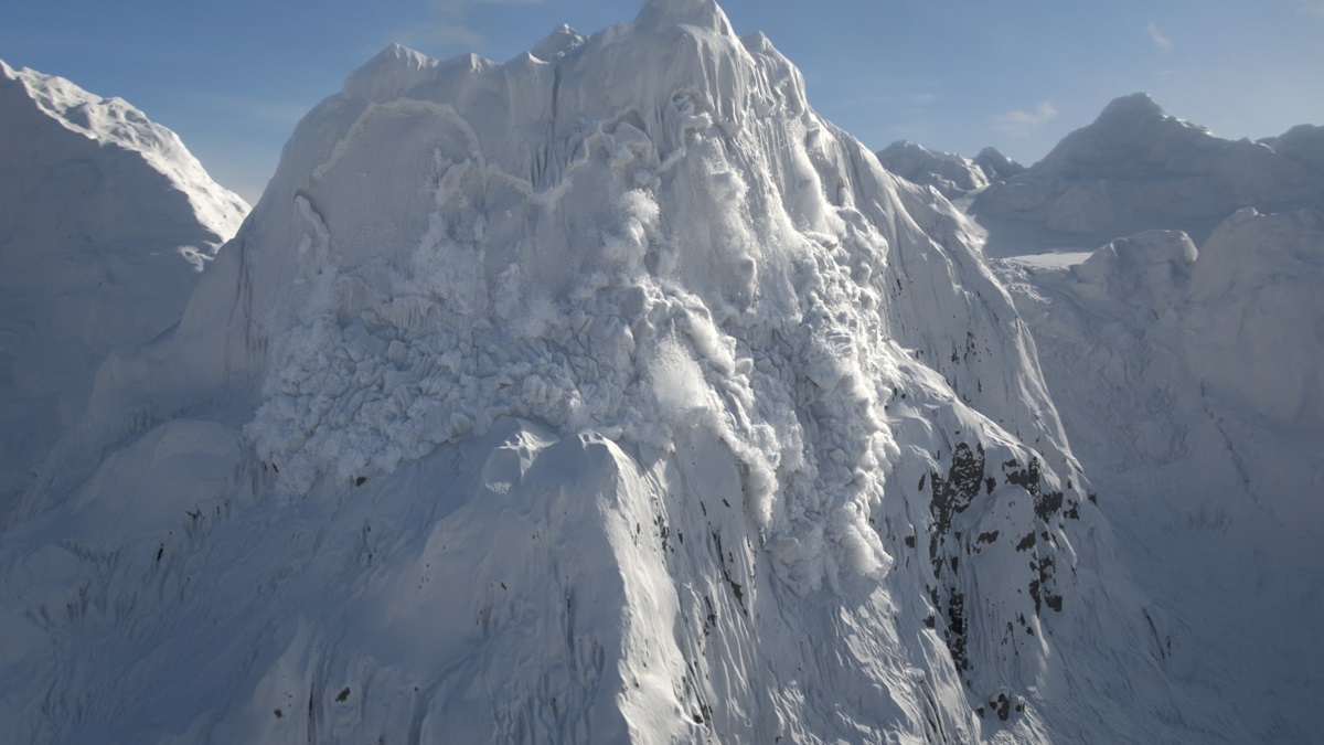
MPM stands for material point method and is an extension of the FLIP Solver to solid mechanics. It allows the simulation of multiple materials such as snow, soil, mud, concrete, metal, jello, rubber, water, honey, and sand. This two-way coupling lets both of the materials affect each other in the same environment.
The implementation is based on OpenCL to leverage the powerful GPUs present in most machines. The background grid uses NanoVDB, which is sparse by default. The rebuilding of the background grid is done on the CPU to free up as much memory as possible on the GPU.
MPM makes dynamic fracturing realistic and easy, but everything can eventually break. It can use multiphysics (provided all things are MPM), and is really good at simulating clumpy/chunky materials. It uses a SOP-based workflow, with the option of user defined forces with a dive target. The typical node tree is made up of the following parts.
MPM components 
Defines the material points to be injected in the MPM simulation. This node creates points and sets material point attributes that can be manipulated to add variation on a per-point basis before going into the ![]() MPM Solver. It expects a mesh or volume as input, and fills the object with particles holding the material attributes. Many MPM Sources can be merged together before they are passed to the MPM Solver.
MPM Solver. It expects a mesh or volume as input, and fills the object with particles holding the material attributes. Many MPM Sources can be merged together before they are passed to the MPM Solver.
Defines colliders to be used in the simulation. Only VDB colliders are supported. This node can create the VDB representation from a mesh or be provided with a VDB directly. Three types of colliders are supported: static, transformed, and deforming. Many MPM Colliders can be merged together before they are passed to the MPM Solver.
Defines the resolution and start frame of the MPM simulation. For this reason, it must be known by all MPM nodes involved in the solve. The ![]() MPM Source,
MPM Source, ![]() MPM Collider, and
MPM Collider, and ![]() MPM Solver all have an input to be connected to this node. This can optionally be done with a dependency link in the MPM Container parameter on these nodes. If you choose to do this, make sure you have Show for Selected Nodes turned on in the Dependency Link section of the View menu in the network editor. You can optionally add boundaries to the simulation container. By default the container is unbounded, but it can be useful to define some limits where material particles are bounced or deleted on contact.
MPM Solver all have an input to be connected to this node. This can optionally be done with a dependency link in the MPM Container parameter on these nodes. If you choose to do this, make sure you have Show for Selected Nodes turned on in the Dependency Link section of the View menu in the network editor. You can optionally add boundaries to the simulation container. By default the container is unbounded, but it can be useful to define some limits where material particles are bounced or deleted on contact.
Does the actual work of solving the scene based on the sources and colliders passed to its first and second inputs respectively. It can simulate many material types in a multi-physic context. MPM is an extension of FLIP to solid mechanics that was first introduced to graphics to simulate snow. It is particularly efficient at solving elastoplastic “chunky” materials where large chunks are expected to stick together, such as snow and soil. It is also possible to simulate complex interactions like water carrying large chunks of soil or concrete. It is also where you control the substeps and ground plane.
See MPM Workflow for more information.
MPM network layout 
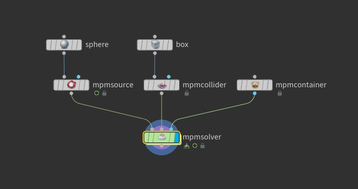
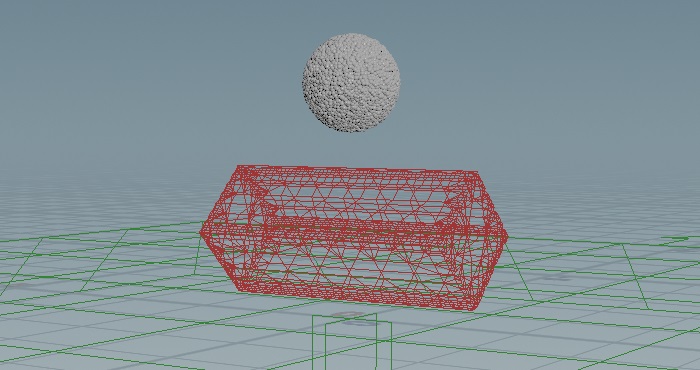
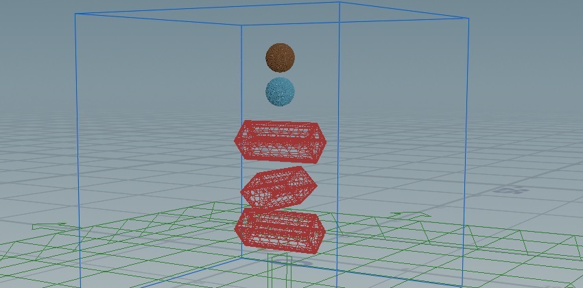
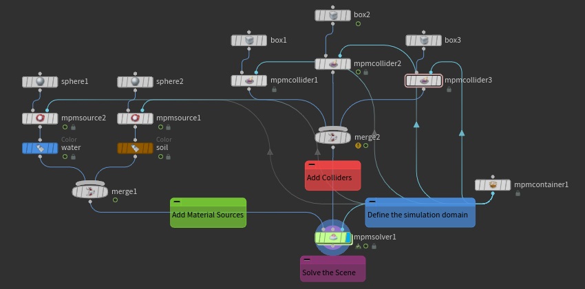
You can use the tab menu to put down an MPM Configure for an example of a simple setup. The first branch is the MPM Source, which defines the material you're going to simulate. The second branch is the MPM Collider, which can either be animated or static. The third branch is the MPM Container, which defines the resolution of the simulation and sets limits on whether particles should be deleted or bounce on contact. All of these 3 components feed into the MPM Solver, which does the work of solving the scene.
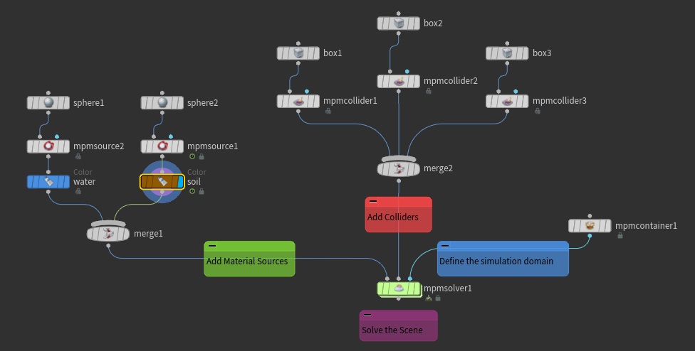
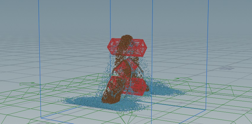
You can optionally merge multiple sources or colliders into one stream before feeding them into the MPM Solver. The following example shows soil and water colliding with two static and one animated piece of geometry.
Note
The container must be referenced in the MPM Container parameter on all source and collider nodes. You can do this by using the ![]() Operation Chooser dropdown menu, or by dragging the node from the network to the parameter field. Optionally, you can connect it to the second input for each node; however, this could make the network look more cluttered.
Operation Chooser dropdown menu, or by dragging the node from the network to the parameter field. Optionally, you can connect it to the second input for each node; however, this could make the network look more cluttered.
There are also other MPM Configure examples where you can put down more complex networks using the different material types. See MPM Configure Examples for more information.