| On this page |
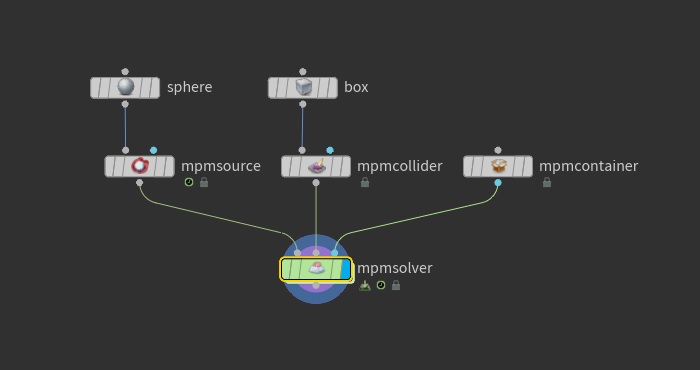
MPM networks are made up of 4 components: ![]() MPM Source,
MPM Source, ![]() MPM Collider,
MPM Collider, ![]() MPM Container, and
MPM Container, and ![]() MPM Solver. The set up is pretty straightforward, as the first three nodes are wired into the solver, respectively.
MPM Solver. The set up is pretty straightforward, as the first three nodes are wired into the solver, respectively.
MPM Source 
The ![]() MPM Source creates MPM particles from a geometry mesh or volume and defines the material type to be used for the simulation. The Material Preset parameter is the most important one to be aware of when first putting down this node. It provides you with a selection of preset materials to quickly get a starting point when setting up a new simulation. These include the following material types: snow, soil, mud, concrete, metal, jello, rubber, water, honey, and sand. Different materials types will be slower or faster to simulate. For example, concrete is much stiffer than snow or water, so it requires more substeps and takes longer to simulate. If you have multiple source materials in the same simulation, the number of substeps will be driven by the stiffest material.
MPM Source creates MPM particles from a geometry mesh or volume and defines the material type to be used for the simulation. The Material Preset parameter is the most important one to be aware of when first putting down this node. It provides you with a selection of preset materials to quickly get a starting point when setting up a new simulation. These include the following material types: snow, soil, mud, concrete, metal, jello, rubber, water, honey, and sand. Different materials types will be slower or faster to simulate. For example, concrete is much stiffer than snow or water, so it requires more substeps and takes longer to simulate. If you have multiple source materials in the same simulation, the number of substeps will be driven by the stiffest material.
The next thing you will want to set is whether or not the emission occurs Once, or is Continuous using the Emission Type dropdown menu.
MPM Collider 
The ![]() MPM Collider has three collider types: static, transforming, or deforming. You can also choose whether the material is bounced or deleted once it hits the collider. It is important to note that only VDB colliders are supported. This node can create the VDB representation from a mesh or be provided with a VDB directly.
MPM Collider has three collider types: static, transforming, or deforming. You can also choose whether the material is bounced or deleted once it hits the collider. It is important to note that only VDB colliders are supported. This node can create the VDB representation from a mesh or be provided with a VDB directly.
| To... | Do this |
|---|---|
|
Set up a static collider |
Set the Collider Type is set to Static. This is the default MPM Collider, as it is the most efficient. It is represented by a single VDB |
|
Set up a transforming collider |
This is the most efficient of the animated colliders and it is extremely accurate as the transformation is interpolated between frames for each substep. It is represented by a single VDB along with a transformation matrix. Only the rigid transformation is updated per frame as the VDB |
|
Set up a deforming collider |
This should only be used over the Animated (Rigid) type when actual deformation is taking place, as it is the most expensive of the two. It is represented by a pair of |
|
Make the material stick to the collider |
In the Material section, there are Friction and Sticky parameters. Increasing the value of the Sticky parameter to For an example of this, use the tab menu to put down the MPM Configure Rolling Snowball example. |
MPM Container 
The ![]() MPM Container defines the resolution and start frame of the MPM simulation, which means it must be connected to all MPM nodes involved in the solve. The
MPM Container defines the resolution and start frame of the MPM simulation, which means it must be connected to all MPM nodes involved in the solve. The ![]() MPM Source,
MPM Source, ![]() MPM Collider, and
MPM Collider, and ![]() MPM Solver all have an input to be connected to this node. This can optionally be done with a dependency link in the MPM Container parameter on these nodes. If you choose to do this, make sure you have Show for Selected Nodes turned on in the Dependency Link section of the View menu in the network editor.
MPM Solver all have an input to be connected to this node. This can optionally be done with a dependency link in the MPM Container parameter on these nodes. If you choose to do this, make sure you have Show for Selected Nodes turned on in the Dependency Link section of the View menu in the network editor.
The parameters in the Resolution section are very important, because this is where you set the global particle separation used to drive the resolution of the whole simulation. The Particle Separation parameter not only sets the level of detail for the source, but also the collider. The Grid Scale parameter multiplies the Particle Separation to define the voxel width dx of the background grid. The default of 2 will pack 8 particles per voxel on average.
You can optionally add boundaries to the simulation container. By default the container is unbounded, but it can be useful to define some limits where material particles are bounced or deleted on contact. You can do this in the Boundaries section of the node.
MPM Solver 
The ![]() MPM Solver does the actual work of solving the scene based on the sources and colliders passed to its first and second inputs respectively.
MPM Solver does the actual work of solving the scene based on the sources and colliders passed to its first and second inputs respectively.
There are two types of substeps on this node: Global Substeps and Substeps Min/Max. The Global Substeps are the number of DOP substeps for each simulated frame. This should generally be kept to 1 for performance reasons, but could be increased to achieve smooth continuous emission. The Substeps Min/Max set limits on the minimum and maximum number of substeps. The solver dynamically picks the lowest substep count based on the type and speed of the material. Although the max value is set at 10,000 by default, it doesn’t mean 10,000 are necessarily being used. You can see the actual substep count on the outputted geometry as a detail attribute. The high default value is to account for stiffer materials, like concrete or metal, that will require more substeps and are expected to be slow.
You can optionally apply forces like gravity, air resistance, and wind in the Forces section. You can also turn on a ground plane that have extra parameters to control friction and stickiness, which is useful if you want to simulate something like snow sliding down a slope.
The parameters on the Visualize tab let you see the container, colliders, ground plane, and background grid.
You can also dive inside the The ![]() MPM Solver and add custom forces. This network will be evaluated once per frame. When possible, using Gas OpenCL nodes should lead to better performance than VEX nodes as it will prevent unnecessary copies from the host to the OpenL device.
MPM Solver and add custom forces. This network will be evaluated once per frame. When possible, using Gas OpenCL nodes should lead to better performance than VEX nodes as it will prevent unnecessary copies from the host to the OpenL device.
For more information, see the Troubleshooting page.